CoKon 59

A MAGYAR MITTEILUNGEN TUDOMÁNYOS AKADÉMIA DER CSILLAGVIZSGÁLÓ STERNWARTE INTÉZETÉNEK DER UNGARISCHEN AKADEMIE KÖZLEMÉNYEI DER WISSENSCHAFTEN BUDAPEST-SZABADSÁGHEGY Nr. 59 E. ILLÉS-ALMÁR AND I. ALMÁR PERIOD CHANGES OF THE SATELLITE 1960 EPSILON 3 IN 1963/64 AS DEDUCED FROM OBSERVATIONS WITHIN THE INTEROBS PROGRAM BUDAPEST, 1965 PERIOD CHANGES OF THE SATELLITE 1960 epsilon3 IN 1963/64 AS DEDUCED FROM OBSERVATIONS WITHIN THE INTEROBS PROGRAM* by E. ILLÉS-ALMÁR and I. ALMÁR Zusammenfassung. Aus [7] wurden die Beobachtungen des Satelliten 1960 epsilon3 (Kabine Sputnik 4) ausgewählt und die besten 39 Durchgänge, die sich zwischen 21 August 1963 und 27 Sept. 1964 verteilen, bearbeitet. Zuerst berechnete eine elektronische Rechenmaschine nach der Methode [9] die zu 393 simultanen Vermessungen gehörigen XYZR Raumkoordinaten des Satelliten. Dann wurde (nach einem Vorschlag von I. D. Shongolowitsch) bei jedem Durchgang die Durchgangszeit des Satelliten über einen ausgewählten geographischen Breitenkreis bestimmt (Tab. 3). Insofern die Periode sich gleichmässig änderte, konnte die Beschleunigung pro Umlauf dP/dn mittels der Abweichungen zwischen den beobachteten und den mit einer konstanten Periode berechneten Durchgangszeiten bestimmt werden. Es wurden für 31 Durchgänge (267 Raumpunkte enthaltend) Periodenänderungen dP/dn berechnet (Tab. 4). In allen beobachteten Zeitabständen war die Periodenänderung konstant, mit Ausnahme der ersten, wo am 26 August 1963 der |dP/dn| Wert - parallel mit einer Verminderung der Sonnenfleckenzahl und der Gesamtfläche der Sonnenflecken - plötzlich abgenommen hat (Tab. 5, Abb. 2-8). Diese Änderung war sechsmal grösser als der Standardfehler der vorherigen dP/dn Werte und entsprach einer Verminderung der Luftdichte in der Perigeumhöhe (255 km) um 31%. Es ist bemerkenswert, dass die |dP/dn| Werte in Juli und Sept. wesentlich kleiner waren als die früheren. Diese Verminderung konnte auch unabhängig davon durch den zeitlichen Verlauf der Umlaufszeit bewiesen werden. Dieser Umstand hängt wahrscheinlich auch mit der Abnahme der Sonnenaktivität zusammen und daraus folgt der prolongierte Untergang des Satelliten. INTRODUCTION Air drag is playing a vital role among perturbing forces acting upon the motion of artificial satellites. Its effect becomes visible in the decrease of a, e and the period of revolution (P), these changes being connected with air density in the region near perigee. The decrease of the nodal period of revolution, easily measurable by observing the satellite's reappearance above a given geographic latitude, yealds a suitable tool for the investigation of the influence of air drag on satellite motion. As the deviations between observed and calculated transit times (O-C), on the one hand, and the rate of period * Paper presented at The International Symposium on Satellite Tracking (October 14-17, 1965, Budapest.) change, on the other hand, are closely connected, even a regular tracking network of comparatively small extent might produce valuable data for atmospheric physics. Experience shows, however, that the density of upper atmosphere depends on the intensity of solar activity, hence satellite orbit studies may lead to a better understanding of geophysical influences of the Sun in general. Several successful attempts have been made to utilize optical obser- vations - including also rough visual fixes available in large quantities - in order to investigate changes in the orbital elements of artificial satellites [1]. As optical observations in the general case give only the direction of the satellite with respect to the tracking station, the determination of orbital elements is usually carried out by means of classical celestial mechanics based on a set of observations and on the method of successive approximation (Laplace, Gauss). From an adequate number of optical fixes orbital elements can be obtained, referring to the whole time interval during which the observational material has been collected. The method is more effective if the material is of higher accuracy, more extensive, and covers a longer portion of the whole orbit [2]. In practice, however, because of the quick changes in the elements of artificial satellites due to deviations of the Earth's gravitational field from a central field and also due to air drag, some assumptions must be introduced concerning the direction and speed of changes in the orbital elements in the period under investigation. If perfect synchronism of observations carried out from a base line of appropriate length on the same satellite can be guaranteed in some way or another, the instantaneous position in space of the satellite is fixed. In this case orbit studies which are based on a limited number of observations are possible. This possibility means, in a fortunate case, a shorter time interval during which the shift of orbital elements may be either easily taken into account or neglected. This fact, important mainly for low-orbit satellites, gives an opportunity of studying even quick changes of certain orbital elements (e.g. period of revolution). The synchronism of optical fixes may be assured, in general, by several methods: a). If short light signals are emitted by a satellite at definite times (e.g. ANNA-1B), the position of the satellite with respect to the stars can be photographed from stations at both ends of a base line. This is the best solution of the problem, but owing to technical difficulties it cannot be used frequently. b) If the camera control systems are connected so that they are activ- ated by the same time signal, then every satellite illuminated by the sun can be photographed simultaneously from the tracking stations. The drawback of the method is that this perfect synchronism encounters serious technical difficulties. c) If the apparent path of the satellite is supposed to be a great circle, pairs of simultaneous observations may be selected quite independently of time statements [3]. The topocentric radius vector M_2S belonging to a given topocentric radius vector M_1S must lie, however, in the plane defined by the known radius vector M_1S and the base line M_1M_2, and also in the, plane described by the apparent path of the satellite (notations see on Fig. 1). The line of intersection of these planes fixes the direction of the satellite from M_2 at a specified moment. One drawback of this method is that it requires extensive calculations. d) An interpolation can be used to select a pair of simultaneous observ- ations, frequent and consecutive from at least one of the stations and sporadic from the other, occurring within the same time interval. It is well known that the apparent orbit of an artificial satellite is quite smooth within an interval of less than a minute. Therefore this method has the advantage of reducing the random errors in the observations, since the interpolated values represent mean values of a set of observed azimuthal or equatorial coordinates, provided the orbit is smooth. The method was used in both the Soviet and American triangulation programs [4], [5]; it has been introduced by M. Ill to visual observations [6]. In order to increase the number of simultaneous observations a special network of Hungarian, German, later Soviet, Bulgarian, Polish and Roumanian tracking stations was established in 1961/62 under the designation INTEROBS. It has been organized, according to its coordinator Mr. M. Ill, for the purpose of performing serial observations within previously fixed time intervals on certain artificial satellites. All observations obtained during these intervals („campaigns") were summarized and published at Baja (Hungary) [7]. Several methods have been suggested [8] to evaluate simultaneous observations selected from this material by means of graphic interpolation. The aim of the present paper is to investigate tracking data on the cabin of Sputnik 4 (1960 epsilon3) using a combination of methods proposed at the conference of satellite observers at Riga in 1965. Our experiences have shown that the observational material of the first INTEROBS cycles, collected mainly in Eastern Europe, did not enclose a portion of the orbit long enough to allow exact determination of all orbital elements (e and omega in particular) separately for every revolution. Hence, follow- ing a proposal of I. D. Zhongolovich, we intended only to study the changes of the nodal period of revolution of the satellite. From the material available simultaneous observations carried out in the following intervals have been selected: 21-30 Aug. 1963, 17 Feb., 10-13 Apr., 8-13 June, 7-12 July and 18-27 Sept. 1964. Evaluation has been limited to the following transits: TABLE 1 Dates No. of transit Number of sim. pairs in [7] of observations 1963 21 Aug. 2 6 22 4 15 23 5 9 23 6 18 24 7 1 24 8 8 25 9 2 26 12 9 27 13 8 27 14 4 TABLE 1 (cont.) No. of transit Number of sim. pairs Date in [7] of observations 29 16 12 29 17 5 30 19 5 1964 17 Feb. 27 14 10 Apr. 38 1 10 40 1 11 42 22 12 46 32 13 49 5 8 June 71 4 9 77 3 11 83 1 12 85 17 13 89 3 13 92 1 7 July 93 28 8 94 21 9 95 27 10 96 6 12 98 18 18 Sept. 118 10 20 119 12 22 120 9 22 122 16 23 123 7 24 127 2 25 128 5 26 134 8 27 138 18 Total: 39 transits 393 simultaneous points The contribution of tracking stations to the observational material is the following TABLE 2 Country Station Number of number fixes Ryazan U.S.S.R. 1042 136 Baja Hungary 1113 124 Budapest Hungary 1111 84 Vologda U.S.S.R. 1014 84 Arkhangelsk U.S.S.R. 1004 80 Cluj Roumania 1132 47 Chernovtsy U.S.S.R. 1062 45 Riga U.S.S.R. 1040 36 Kiev U.S.S.R. 1023 29 Kishinev U.S.S.R. 1024 27 Bautzen G.D.R. 1120 21 TABLE 2 (cont.) Country Station Number of number fixes Tartu U.S.S.R. 1051 17 Olsztyn Poland 1151 17 Rostov U.S.S.R. 1041 14 Rodewisch G.D.R. 1185 8 Erevan U.S.S.R. 1018 7 Dnepropetrovsk U.S.S.R. 1017 5 Stara Zagora Bulgaria 1102 5 Birsk U.S.S.R. 1085 4 Kazan U.S.S.R. 1020 1 Petrozavodsk U.S.S.R. 1038 1 Zvenigorod U.S.S.R. 1072 1 Total: 22 stations 793 fixes. Plotting the celestial coordinates against time, pairs of simultaneous observations have been selected by the aforementioned method of graphic interpolation. If serial fixes were made from several stations at the same time, we tried to adopt the procedure of interpolation on the sequences of each station. Single observations are weighted by 1; coordinates interpolated at the beginning or at the end of a sequence (uncertain values) by 2; reliably interpolated values by 3. The authors would like to thank Mr M. Ill and Mr K. Süto for kindly permitting the use of pairs of simultaneous points selected by them from the material of the Aug. 1963, Feb. and Apr. 1964 intervals. THE METHOD Instantaneous positions in space of the satellite have been determined from pairs of simultaneous fixes according to the procedure proposed at the Riga conference [9]. Its program used in the computer reduction (electronic computer Type Elliott 803) is given in the Appendix. Starting from observations in the equatorial coordinates (alpha_1 delta_1 and alpha_2 delta_2 respectively) equations are written for planes in a rectangular system fixed in space, satisfying the following two conditions: a) they each contain one observing station, M_1 or M_2; b) they contain angles alpha_1 and alpha_2 with the [XY] plane of the coordinate system respectively. The coordinates x_s and y_s of the satellite are given by the line of intersection of the planes (mu). If straight lines are drawn inside these planes containing the angles 90° - delta_1, 90° - delta_2 (measured from the North Pole) from stations M_1 and M_2 respectively, their intersection with mu provides two fictitious positions of the satellite in space (S_I, S_II) (see Fig. 1). Forming their appropriately weighted mean value, points in space can be obtained which

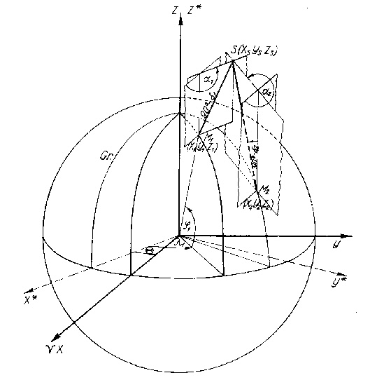Fig. 1. serve as a basis for further calculations (S_1, S2,...). The set of equations used is a simple consequence of the basic equation of cosmic triangulation [10]:

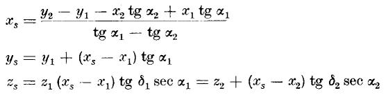It is to be noted that the method offers the advantage of providing a pair of solutions even in the case of not absolutely accurate observations (without a least-squares solution), as the errors in the initial data present themselves in the deviation of the two different results for the z_s coordinate of the satellite. The use of serial fixes makes a graphic smoothing of the x_s, y_s, z_s and

values feasible. I. D. Zhongolovich proposed in a paper presented at the Riga conference under the title "Remarks to the Interobs program" that changes of the nodal period of revolution of satellites should be determined from the visual observations. He proved that sequences of spatial positions give transit times above a given geographic latitude circle (phi_0) accurate to at least a few tenths of a second. Consequently from two passes observed on two consecutive nights the mean period of revolution of the satellite is determinable to a few hundredths of a second. There is hereby a hopeful possibility to analyse quick period changes of low-orbit satellites with an adequate accuracy. First of all the geocentric latitude of the subsatellite points (phi_n) is needed. It can be easily derived from space coordinates, namely through

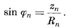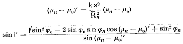
Plotting phi_n, as a function of the epoch of observation (t_n) we are able to perform on the smoothed curve a graphic determination of the satellite's crossing time over the given latitude circle (t_0). The numerical procedure proposed by Zhongolovich is more accurate and makes extrapolation possible. If the path element in question is short, equation

holds true, where

if R_n and a are expressed in kilometers, (t_n - t_0) in seconds and (mu_n - mu_0) in degrees. Calculating the transit times t_0 belonging to phi_0 from every pair (t_n phi_n) separately, their mean value

is to be formed. As a first step, however, approximate values of i, a and e are needed. Orbital elements published by prediction services might be used as a first approximation. Taking them as a starting point, all t_0 values on a selected long transit of high quality should be calculated. If the t_0 values thus obtained show a monotonous decrease or increase as a function of time, the adopted value of i has to be corrected. To derive its correct value we may proceed as follows: if e.g. t_01 < t_0 < t_02 where t_01 and t_02 are arbitrary t_0 values at the beginning (t_n1) and at the end (t_n2) of the given transit respectively, we have

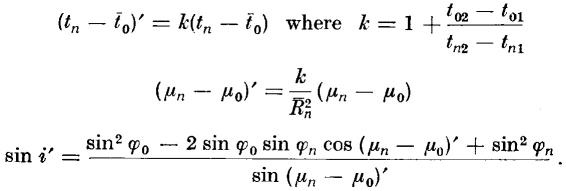Dashed letters are the corrected quantities. A mean value of i', derived from several pairs of (t_n1, t_n2) equals the correct inclination of the orbital plane. Then follows the determination of a using

values of a pair of well observed transits separated by nearly 24 hours

. With the approximate value of the orbital period, the revolution number (n) between the two selected transits can be guessed. Hence we get

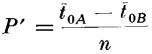the nodal period of revolution in a closer approximation. Kepler's third law then yields a (the deviation between nodal and sidereal period of revolution is not significant - see later) and combining it with e we obtain kappa. The value of e can be easily estimated if there are observations near perigee or apogee (i.e. R_per or R_ap is known), because then

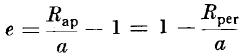will hold. Finally, using the corrected i and kappa values, the calculation of t_0 from every point of every transit has to be completed. It is advisable to choose phi_0 inside or at least near to the observed portions of the orbits in question, but experience shows that it is acceptable also if subsatellite points are not farther from the selected latitude circle than 6-8 degrees. The mean value of the t_0 values represents the observed crossing time over the latitude phi_0 during a given transit:

For organizational reasons, as a rule, Interobs cycles lasted 7-10 days per month, therefore period changes were investigated within each cycle separately. Calculations may be carried out as follows. Let us suppose as a first approximation that the period is constant and equals to its approximate value, P', furthermore that the starting epoch

Plotting the O - C values against time, usually a parabola is obtained, in accordance with the general tendency of decreasing of the period of revolution. Then the P_0 period, belonging to the first of the transits observed, is to be determined, using either graphic or - following a proposal of M. Ill - numerical solution. He supposes that during the given time interval nodal period increases steadily by Delta sec per each revolution, then

where

and the period changes during one revolution by

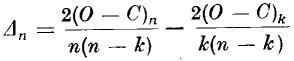where (O - C)_k belongs to the k^th, (O - C)_n to the n^th orbit and

n > k. For practical purposes two well observed transits should be selected. Repeating the calculation of residuals using the P_0 value from either the graphic or the numerical solution we have

which yields as a result the rate of change of the nodal period for each transit separately

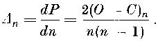If these results are equal, i.e. Delta_n = const., our assumption appears to be valid and the procedure yields the period change in the whole interval in question. If Delta_n varies, we should try to divide the interval into several parts and select points near enough to each other to allow the determination of a Delta_n = const. value. In practice it may seem reasonable to plot first 2(O - C)_n as a function of n(n - 1) and test whether the points lie on a single straight line or not. If it can be assumed that Delta_n = const., it is worth while to carry out the inverse procedure, namely to determine P_z, the period of revolution belonging to the last transit of the interval. Then in the opposite direction

hence Delta_m can be calculated exactly in the same manner as in the previous case. The influence of the errors of the observed O_n values on Delta_n being inversly proportional to n(n - 1), we formed a weighted mean of the Delta_n and Delta_m pairs for every transit separately

The result has been considered as the rate of decrease of the period (in sec/rev) during the time interval under consideration. RESULTS The part of the observational material published in [7], seemingly most suitable to an investigation of the type outlined above, consisted of 39 transits of 1960 epsilon3. Altogether 6 transits have been rejected, partly because the path element observed was too far from the latitude circle phi_0 (pass No. 5), partly because it belonged to a time interval where the number of suitable transits to deduce period changes proved to be insufficient (pass No. 27 and passes No. 77, 83, 89, 92 respectively). One third of all positions in space, given by the computer program, have been similarly neglected (126 points out of 393). These points have been rejected because a) they belong to transits already cancelled; b) they were far from the latitude circle phi_0; c) the length of their radius vector, R, differed considerably from all other R values of the transit (in some cases it is a consequence of the decreased parallax of the satellite as seen from the pair of stations); d) another set of XYZR values could be derived from other observations but referring to the same moment. In this case corresponding quantities have been averaged. A review of the whole observational material is given in Table 1. Positions in space actually used, the partial results of the Zhongolovich method and transit times are summarized in Table 3. TABLE 3 t_n z_n R_n t_0-t_n t_0 h m s km km s h m s 1963 21.8 20 34 2.8 6020. 6858.83 20.1 20 34 22.9 34 6.7 6010.5 6848.37 19.9 34 26.6 22.8 21 4 17.9 6110.43 6859.57 81.2 21 5 39.1 4 31.4 6090.99 6861.64 64.9 5 36.3 4 36.4 6087.69 6861.62 62.5 5 38.9 4 40.2 6082.55 6861.98 58.7 5 38.9 5 3.7 6052. 6863. 37.6 5 41.3 5 5.3 6048. 6864. 34.5 5 39.8 5 27.2 6015.09 6862.84 15.3 5 42.5 6 5.0 5942. 6866. -25.1 5 39.9 6 24.0 5902.50 6867.69 -44.7 5 39.3 6 34.2 5878.51 6866.34 -55.1 5 39.1 6 44.0 5853.54 6862.84 -64.7 5 39.3 23.8 20 3 43.9 6094.75 6857.87 70.2 20 4 54.1 3 51.9 6082.94 6855.64 62.9 4 54.8 4 3.1 6062.33 6856.60 47.9 4 51.0 4 5.8 6060.84 6855.22 47.7 4 53.5 4 30.0 6022.95 6857.82 22.4 4 52.4 4 43.4 6001.38 6860.18 8.8 4 52.2 4 58.7 5974.39 6859.39 -5.6 4 53.1 5 5.0 5970.77 6874.76 -10.0 4 55.0 5 46.5 5874.21 6858.28 -53.8 4 52.7 6 5.0 5833.03 6859.42 -72.2 4 52.8 24.8 19 4 0.2 5741.15 6588.34 3.7 19 4 3.9 20 34 57.6 6083.11 6851.52 65.6 20 36 3.2 35 15.1 6058.43 6853.67 47.0 36 2.1 35 17.8 6054.62 6851.09 46.0 36 3.8 35 38.5 6024.46 6856.65 23.9 36 2.4 36 29.0 5932.74 6858.58 -26.5 36 2.5 25.8 19 34 4.3 6103.25 6865.52 71.6 19 35 15.9 36 28.6 5831.57 6879.74 -80.5 35 8.1 26.8 20 5 26.8 6062.73 6859.66 46.4 20 6 13.2 5 30.4 6058.48 6858.20 44.5 6 14.9 5 32.7 6055.18 6857.24 42.8 6 15.5 5 33.3 6054.48 6857.11 42.5 6 15.8 5 40.4 6044.36 6855.46 36.9 6 17.3 6 0.4 6012.86 6856.22 17.3 6 17.7 7 39.0 5808.94 6855.04 -80.6 6 18.4 27.8 19 5 14.4 6000.01 6855.34 10.4 19 5 24.8 5 52.1 5938. 6858.99 24.1 5 28.0 6 4.0 5912.84 6874.50 -42.7 5 21.3 TABLE 3 (cont.) t_n R_n t_0-t_n t_0 h m s km km s h m s 6 5.0 5910.95 6875.98 -44.2 5 20.8 6 39.3 5825.51 6857.24 -74.5 5 24.8 20 36 49.8 6092.35 6928.63 27.3 20 37 17.1 39 3.7 5760.66 6860.36 -101.9 37 21.8 39 4.6 5754.54 6854.32 -102.1 37 22.5 39 5.6 5747.28 6844.68 -101.5 37 24.1 29.8 18 34 32.3 6073.52 6855.59 56.2 18 35 28.5 34 59.1 6032.15 6857.14 28.3 35 27.4 35 3.8 6029.80 6860.94 24.9 35 28.7 35 4.6 6031.07 6863.07 24.6 35 29.2 35 5.5 6032.27 6865.09 24.2 35 29.7 36 3.8 5905.21 6851.47 -36.7 35 27.1 36 4.8 5903.23 6851.77 -37.8 35 27.0 36 6.1 5901.27 6852.49 -39.0 35 27.1 36 10.5 5900.06 6859.18 -42.4 35 28.1 20 7 23.4 5990.36 6862.02 1.8 20 7 25.2 7 49.8 5939.31 6863.97 -25.6 7 24.2 7 52.9 5941.68 6871.21 -27.6 7 25.3 30.8 19 6 34.6 5968.99 6859.71 -8.6 19 6 26.0 6 34.8 5969.20 6859.39 -8.3 6 25.5 1964 10.4 18 14 7.5 5107.44 6753.54 10.6 18 14 18.1 19 46 14.2 5287.86 6780.66 -32.9 19 45 41.3 11.4 18 34 37.2 4888.92 6822.06 78.5 18 35 55.7 34 40.8 4902.36 6817.63 74.4 35 55.2 34 43.3 4910.40 6813.19 71.6 35 54.9 34 44.9 4916.75 6812.34 69.9 35 54.8 34 48.1 4927.56 6806.41 66.2 35 54.3 34 51.0 4940.47 6806.28 63.0 35 54.0 34 52.5 4944.53 6903.25 61.5 35 54.0 34 56.3 4963. 6801.32 56.6 35 52.9 34 59.0 4974. 6795.90 52.8 35 51.8 34 59.6 4976.64 6805.79 54.1 35 53.7 35 2.9 4994.18 6810.19 50.7 35 53.6 35 5.9 5009.50 6813.21 47.6 35 53.5 35 9.8 5027.16 6814.47 43.3 35 53.1 35 11.5 5032.33 6812.09 41.5 35 53.0 35 13.1 5037.87 6810.68 39.9 35 53.0 35 15.8 5047.97 6809.14 37.0 35 52.8 35 18.4 5056. 6802.86 33.7 35 52.1 35 20.8 5059.60 6799.49 32.2 35 53.0 35 24.9 5072.70 6795.92 28.1 35 53.0 12.4 18 57 18.0 5143.25 6781.82 6.9 18 57 24.9 57 23.5 5175.94 6790.47 0.0 57 23.5 57 28.7 5195.29 6790.15 -5.3 57 23.4 57 31.7 5201.69 6786.30 -7.8 57 23.9 57 33.9 5207.49 6786.19 -9.4 57 24.5 57 39.0 5218.91 6779.86 -13.8 57 25.2 57 43.5 5223.77 6770.78 -17.0 57 26.5 57 46.3 5253.41 6785.25 -22.2 57 24.1 57 50.3 5262.79 6780.38 -25.9 57 24.4 57 55.3 5288.62 6786.64 -31.8 57 23.5 1 57 59.4 5299.50 6784.09 -35.5 57 23.9 58 4.6 5312.73 6780.55 -40.0 57 24.6 TABLE 3 (cont.) t_n z_n R_n t_0-t_n t_0 h m s km km s h m s 58 9.4 5325.72 6777.97 -44.3 57 25.1 58 14.0 5340.78 6777.23 -48.9 57 25.1 58 18.8 5358.97 6778.01 -54.0 57 24.8 58 23.4 5376.34 6778.87 -59.0 57 24.4 58 26.9 5387.13 6778.15 -62.4 57 24.5 58 30.8 5400.01 6777.84 -66.4 57 24.4 58 33.8 5408.82 6777.49 -69.2 57 24.6 58 38.8 5414.63 6770.89 -72.4 57 26.4 58 42.8 5430.92 6772.68 -77.0 57 25.8 13.4 17 48 47.6 5426.59 6775.45 10.2 17 48 57.8 48 49.3 5437.17 6775.39 6.9 48 56.2 48 56.8 5458.46 6776.53 0.5 48 57.3 50 14.1 5679.94 6774.16 -76.6 48 57.5 8.6 0 18 36.2 4643.84 6754.14 102.3 0 20 18.5 18 48.4 4697.44 6752.85 90.1 20 18.5 19 1.9 4759.26 6751.10 75.8 20 17.7 19 17.6 4820.83 6747.15 60.8 20 18.4 12.6 0 5 42.0 4933.49 6758.85 36.1 0 6 18.1 6 16.5 5069.15 6749.97 0.4 6 16.9 6 19.1 5069.95 6742.04 -1.3 6 17.8 6 20.5 5084.84 6750.54 -3.5 6 17.0 6 24.6 5100.91 6750.15 -7.8 6 16.8 6 31.2 5125.03 6748.76 -14.4 6 16.8 6 33.1 5133.45 6749.98 -16.3 6 16.8 6 34.6 5125.46 6739.29 -16.3 6 18.3 6 37.6 5134.63 6737.21 -19.2 6 18.4 6 42.6 5143.52 6729.61 -23.0 6 19.6 6 44.7 5175.52 6747.64 -28.1 6 16.6 7 13.4 5216.78 6743.11 -57.1 6 16.3 7 19.2 5287.78 6736.80 -61.5 6 17.7 7.7 0 37 59.6 4860.98 6601.83 -56.2 0 37 3.4 38 0.2 4854.41 6601.74 -55.3 37 4.9 38 3.8 4864.64 6635.36 -59.4 37 4.4 38 3.9 4866.70 6640.38 -59.9 37 4.0 38 7.3 4852.35 6639.35 -63.1 37 4.2 38 10.3 4843.32 6644.37 -66.2 37 4.1 38 12.3 4831.54 6639.01 -68.0 37 4.3 38 16.6 4814.69 6640.10 -72.2 37 4.4 38 18.4 4809.48 6643.77 -74.1 37 4.3 38 20.4 4800.52 6642.09 -75.9 37 4.5 38 22.9 4791.36 6645.93 -78.8 37 4.1 38 24.2 4785.95 6645.32 -80.0 37 4.2 38 26.5 4777.49 6648.37 -82.6 37 3.9 38 28.6 4768.32 6649.01 -84.8 37 3.8 38 33.5 4744.89 6642.83 -89.0 37 4.5 38 34.9 4738.86 6644.81 -90.8 37 4.1 38 42.1 4706.07 6639.95 -97.3 37 4.8 38 44.2 4697.43 6640.31 -99.3 37 4.9 38 47.1 4684.79 6639.51 -102.1 37 5.0 38 47.8 4680.92 6638.97 -102.9 37 4.9 38 50.5 4668.94 6637.18 -105.2 37 5.3 38 56.6 4641.99 6638.00 -111.4 37 5.2 38 59.1 4632.78 6636.94 -113.3 37 5.8 39 1.3 4621.96 6637.93 -115.8 37 5.5 TABLE 3 (cont.) t_n z_n R_n t_0-t_n t_0 h m s km km s h m s 39 6.9 4599.51 6636.37 -120.5 37 6.4 8.7 23 42 45.9 5128.98 6652.95 4.4 23 42 50.3 42 58.8 5067.39 6643.29 -10.0 42 48.8 42 58.9 5073.59 6647.58 -9.3 42 49.6 42 59.6 5072.33 6649.09 -9.9 42 49.7 43 1.3 5055.44 6641.69 -12.8 42 48.5 43 1.6 5063.18 6648.40 -12.1 42 49.5 43 2.8 5068.83 6656.49 -12.3 42 50.5 43 3.3 5056.21 6648.41 -14.0 42 49.3 43 3.8 5043.74 6640.33 -15.6 42 48.2 43 4.5 5054.12 6650.77 -15.0 42 49.5 43 7.3 5019.17 6632.89 -20.4 42 46.9 43 12.0 5000.94 6631.83 -24.9 42 47.1 43 13.3 5004.66 6638.05 -25.2 42 48.1 43 16.8 5003.09 6647.08 -27.4 42 49.4 43 19.0 4998.61 6650.34 -29.2 42 49.8 9.7 22 29 17.5 5277.51 6654.29 45.9 22 30 3.4 29 30.8 5221.53 6643.98 32.0 30 2.8 29 31.1 5229.64 6650.71 31.4 30 2.5 29 32.8 5217.71 6643.07 31.1 30 3.9 29 33.7 5223.84 6650.89 31.1 30 4.8 29 35.5 5217.37 6650.22 29.4 30 4.9 29 47.8 5172.63 6649.83 17.0 30 4.8 29 48.8 5170.49 6649.04 16.6 30 5.4 30 1.5 5124.09 6649.02 3.9 30 5.4 30 1.8 5120.42 6647.84 3.2 30 4.6 30 2.9 5115.17 6648.13 1.7 30 4.6 30 3.5 5113.63 6647.84 1.3 30 4.8 30 4.2 5110.01 6649.05 0.1 30 4.3 30 4.3 5111.41 6651.43 0.0 30 4.3 30 5.6 5103.68 6648.23 -1.4 30 4.2 30 11.0 5081.84 6644.50 -6.4 30 4.6 30 12.0 5072.41 6640.64 -8.1 30 3.9 30 17.7 5063.50 6649.84 -12.4 30 5.3 30 17.9 5062.39 6648.28 -12.3 30 5.6 10.7 22 48 3.4 5187.55 6638.88 23.5 22 48 26.9 48 4.3 5179.83 6634.82 22.1 48 26.4 48 7.4 5174.19 6636.66 20.2 48 27.6 48 15.6 5163.91 6653.04 13.9 48 29.5 48 16.3 5152.48 6647.66 11.9 48 28.2 48 17.3 5137.48 6641.20 9.2 48 26.5 12.7 21 52 27.8 5427.84 6649.54 93.5 21 54 1.3 52 28.8 5425.39 6649.57 92.7 54 1.5 52 29.9 5421.51 6649.09 91.5 54 1.4 52 30.8 5419.21 6649.34 90.7 54 1.5 52 32.0 5415.74 6649.30 89.6 54 1.6 52 32.7 5413.68 6649.39 88.9 54 1.6 52 33.7 5411.67 6659.71 85.8 53 59.5 53 14.1 5281.86 6645.06 49.2 54 3.3 53 19.4 5257.84 6653.90 40.4 53 59.8 53 19.8 5262.27 6647.48 42.9 54 2.7 53 31.1 5211.77 6649.45 27.9 53 59.0 53 32.4 5205.10 6649.63 26.1 53 58.5 53 33.6 5208.04 6648.43 27.2 54 0.8 18.9 2 5 0.6 4954.33 6644.91 -933.9 1 49 26.7 TABLE 3 (cont.) t_n z_n R_n t_0-t_n t_0 h m s km km s h m s 5 2.3 4948.46 6643.43 -934.6 49 27.7 5 29.7 4829.03 6636.74 -960.6 49 29.1 5 32.2 4813.30 6626.59 -959.6 49 32.6 5 34.1 4812.87 6640.79 -966.3 49 27.8 5 45.2 4760.84 6630.23 -973.6 49 31.6 6 5.7 4675.89 6636.61 -996.0 49 29.7 6 11.2 4657.66 6636.95 -1000.2 49 31.0 20.9 17 30 6.1 4926.57 6674.28 112.0 17 31 58.1 30 7.8 4930.97 6671.76 110.4 31 58.2 30 9.7 4938.37 6671.38 108.4 31 58.1 30 19.8 4982.93 6673.96 97.8 31 57.6 30 26.5 4989.78 6658.22 92.7 31 59.2 30 30.7 5031.35 6678.74 86.6 31 57.3 30 49.3 5095.04 6671.35 68.4 31 57.7 30 50.3 5096.26 6669.22 67.6 31 57.9 22.9 16 34 2.6 5477.57 6656.56 -48.7 16 33 13.9 34 3.8 5479.62 6655.14 -49.9 33 13.9 34 4.8 5482.16 6654.74 -50.8 33 14.0 34 5.8 5485.12 6654.91 -51.8 33 14.0 34 6.9 5487.38 6653.99 -52.5 33 14.4 34 7.9 5491.00 6654.71 -53.8 33 14.1 34 35.6 5568.86 6655.83 -81.3 33 14.3 34 36.8 5573.55 6657.15 -82.6 33 14.2 34 38.0 5578.89 6658.95 -84.1 33 13.9 18 3 29.6 5178.92 6668.67 45.1 18 4 14.7 4 2.9 5297.01 6667.70 11.1 4 14.0 4 30.5 5391.38 6668.67 -17.5 4 13.0 4 48.8 5442.07 6664.26 -34.9 4 13.9 4 52.0 5447.39 6664.68 -36.5 4 15.5 4 59.5 5471.38 6662.69 -45.0 4 14.5 5 4.6 5493.56 6666.04 -51.7 4 12.9 5 30.4 5542.81 6649.05 -73.7 4 16.7 23.9 18 21 34.1 5521.20 6642.81 -67.6 18 20 26.5 22 3.2 5574.84 6631.69 -90.5 20 32.7 22 29.5 5618.38 6620.82 -110.8 20 38.7 22 31.3 5700.50 6661.52 -132.1 20 19.2 22 32.5 5700.74 6660.27 -132.6 20 19.9 23 1.0 5823.06 6695.36 -177.3 20 3.7 24.9 18 38 2.4 5608.90 6655.49 -96.5 18 36 25.9 38 34.2 5677.66 6649.56 -126.2 36 28.0 25.9 17 23 1.7 5609.73 6656.91 -96.4 17 21 25.3 23 3.1 5612.12 6655.79 -97.7 21 25.4 23 17.9 5644.91 6650.97 -112.2 21 25.7 23 18.6 5644.74 6648.72 -112.8 21 25.8 23 19.0 5644.56 6647.10 -113.2 21 25.8 26.9 17 39 0.2 5618.85 6667.50 -96.8 17 37 23.4 40 2.3 5742.56 6651.61 -154.4 37 27.9 40 2.7 5742.10 6651.25 -154.3 37 28.4 40 3.1 5743.18 6651.82 -154.6 37 28.5 40 3.6 5746.71 6653.99 -155.5 37 28.1 27.9 16 25 3.7 5764.70 6657.87 -162.6 16 22 21.1 25 4.7 5765.68 6656.70 -163.5 22 21.2 25 5.7 5766.35 6655.23 -164.4 22 21.3 25 6.5 5767.83 6654.72 -165.3 22 21.2 25 32.9 5805.78 6647.18 -187.6 22 25.3 TABLE 3 (cont.) tn z_n R_ t_0-t_n tv h m s km km s h m s 25 33.2 5796.57 6640.98 -185.2 22 28.0 25 33.9 5796.86 6640.72 -185.5 22 28.4 25 35.0 5800.53 6642.86 -186.5 22 28.5 25 35.8 5798.89 6641.80 -186.1 22 29.7 25 36.9 5805.03 6645.17 -188.0 22 28.9 26 4.2 5858.08 6647.43 -217.2 22 27.0 26 5.1 5859.95 6648.00 -218.1 22 27.0 26 6.0 5860.88 6647.78 -218.8 22 27.2 26 6.9 5861.11 6646.86 -219.4 22 27.5 Different kinds of Delta values deduced from 31 passes by graphic or numerical solution are given in Table 4. In the first column "O" means simply the mean of the t_0 values of Table 3, averaged for each revolution separately. In the second column the root-mean-square error of

(expressed in seconds) is given for all transits which include a large enough number of observations. Its average value is 0.656. Note: The epoch O = 496.259943 comes from two O values combined from two consecutive transits, each containing one pair of simultaneous observations only. The next table gives the period at the beginning and at the end of each observation cycle, its mean value, the mean rate of decrease of the period during each time interval, and its standard error. (As dP/dn changed suddenly on 26 August 1963, the first cycle has been divided into two parts.) Then follows, as a comparison, |dP/dN|^*, defined as the slope of a plot of

against t at the cycles of observation. Finally theoretical values of

are given

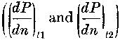calculated from the following equations

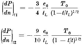[11] where T_0 = 94.27 min., e_0 = 0.030 are initial orbital elements of the satellite, TABLE 4 O sigma Weight (O-C)_n n(n-1) Delta_n (O-C)_m m(m-1) Delta_m

JD 2438... sec day sec/rev day sec/rev sec/rev day 263.357229 +- - 1 - 0 - -.000292 4556 -.0111 -.0111 264.378929 .467 10 -.000012 240 -.0086 -.000161 2652 -.0105 -.0103 265.336725 .389 8 -.000071 930 -.0132 -.000086 1332 -.0112 -.0120 266.294488 - 0.5 -.000162 2070 -.0135 -.000044 462 -.0165 -.0140 266.358366 .309 5 -.000141 2162 -.0113 -.000014 420 -.0058 -.0104 267.316111 - 1 -.000251 3782 -.0115 +.000009 30 +.0518 -.0115 268.337696 .683 7 -.000004 110 -.0063 -.000177 3782 -.0081 -.0080 269.295416 1.320 5 -.000024 650 -.0064 -.000092 2256 -.0070 -.0069 269.359276 - 4 -.000014 702 -.0035 -.000075 2162 -.0060 -.0054 271.274631 .333 8 -.000159 3192 -.0086 -.000010 272 -.0063 -.0084 271.338481 - 3 -.000159 3306 -.0083 -.000003 240 -.0021 -.0079 272.296129 - -.000261 5256 -.0086 - 0 - -.0086 496.259943 - 1 - 0 - -.000168 2162 -.0134 -.0134 497.274926 .237 8 -.000019 240 -.0137 -.000069 930 -.0128 -.0130 498.289868 .186 8 -.000079 992 -.0138 -.000012 210 -.0099 -.0131 499.241334 - 3 -.000178 2162 -.0142 - 0 - -.0142 583.525747 .136 10 - 0 - -.000275 8556 -.0056 -.0056 585.488068 .276 8 -.000027 930 -.0050 -.000117 3782 -.0053 -.0053 586.437551 .194 9 -.000067 2070 -.0056 -.000068 2162 -.0054 -.0055 587.450319 .486 4 -.000123 3782 -.0056 -.000029 930 -.0054 -.0056 589.412511 .389 8 -.000279 8556 -.0056 - 0 - -.0056 656.576036 .582 3 - 0 - -.000781 22952 -.0059 -.0059 659.230532 .200 8 -.000068 1722 -.0068 -.000416 11990 -.0060 -.0061 661.189746 .197 9 -.000175 5256 -.0058 -.000203 6162 -.0057 -.0057 661.252945 .448 5 -.000180 5402 -.0058 -.000198 6006 -.0057 -.0057 662.264160 4.994 0.5 -.000227 8010 -.0049 -.000080 3782 -.0037 -.0045 663.275312 - 1 -.000338 11130 -.0053 -.000026 2070 -.0022 -.0048 664.223213 .105 5 -.000496 14520 -.0059 -.000029 930 -.0054 -.0059 665.234344 .971 4 -.000627 18632 -.0058 -.000005 210 -.0041 -.0058 666.182243 .865 3 -.000787 22952 -.0059 - 0 - -.0059 TABLE 5 Date P_0 day P_z

dP/dn sigma (dP/dn)* (dP/dn)_t_1 (dP/dn)_t_2 day day day sec sec sec sec Aug 1963 I. .0638570 .0638443 .0638506 -.0110 +-.0006 -.0101 -.0072 -.0084 Aug 1963 II. .0638570 .0638443 .0638506 -.00755 .00049 -.0101 -.0072 -.0084 Apr 1964 .0634376 .0634303 .0634340 -.0132 .0003 -.0092 -.0089 -.0103 Jun 1964 - - .0633376 - - - - - Jul 1964 .0633015 .0632956 .0632986 -.00550 .00006 -.0075 -.0098 -.0113 Sep 1964 .0632039 .0631936 .0631987 -.00582 .00020 -.0068 -.0109 -.0126 TABLE 6 Date i e kappa phi_0 mu_0 U_s a h_ap h_per min km km km Aug 1963 64.94 .0173 1723.73 60.750 74.394 92.001 6750.80 490 256 Apr 1964 64.98 .0152 1721.87 49.662 57.264 91.401 6721.45 445 241 June 1964 64.98 .011 1721.34 - - 91.264 6714.70 411 263 July 1964 64.98 .011 1721.32 50.217 58.000 91.208 6711.96 408 260 Sept 1964 64.97 .0104 1720.85 53.131 61.996 91.064 6704.89 397 256 and t_L its total lifetime. Orbital elements in the predictions for March 1965, using the inverse form of the equations quoted above, yielded lifetimes 1874 days and 1896 days respectively. (The actual lifetime of the satellite proved to be somewhat longer.) Figures No 2-8 have been plotted to illustrate the graphic solution of the problem. On Fig. No 2, 4, 5 and 7 deviations between observed and

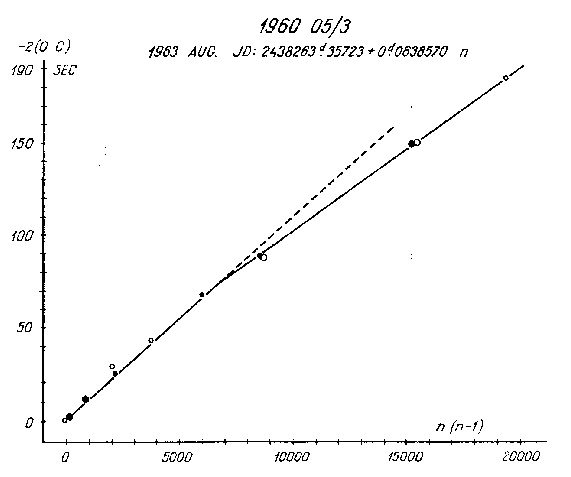Fig. 2. calculated transit times (O - C)_n are plotted against n(n - 1); the slope of each straight line gives Delta_n. C_n values have been derived using the initial period of revolution P_0 and the starting date O_0. Fig. 2 proves clearly the reality of the sudden change which occurred on or about the 26 August. Dashed lines indicate (dP/dn)_t_1 and (dP/dn)_t_2 respectively. (There is certainly a wide gap between the observed and the theoratical values.) Weights of singular points are marked on each of the figures by [big filled circle] [small filled circle] [big circle] [small circle] (in decreasing order). Parameters of major importance for the computations are summarized in the first columns of Table 6 (i, e kappa and phi_0 mu_0, latters representing the reference latitude). Approximate orbital elements have been found in [12] and have been corrected according to the method mentioned above.

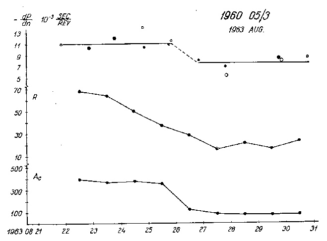Fig. 3.

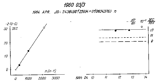Fig. 4.

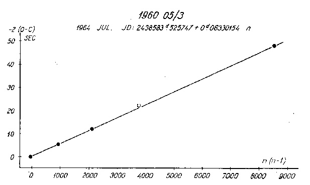Fig. 5.

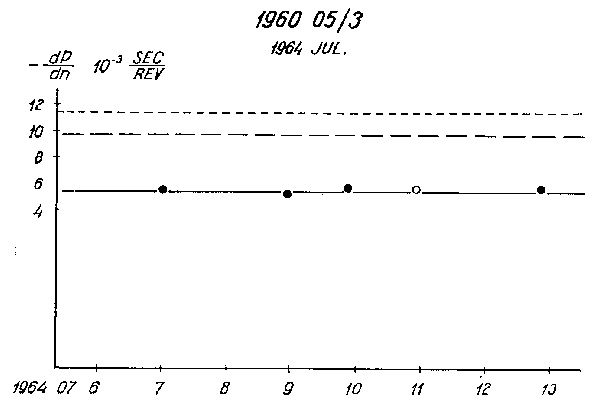Fig. 6.

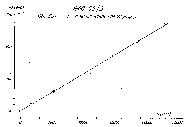Fig. 7.

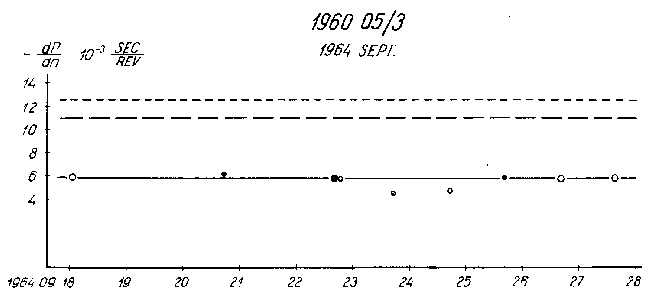Fig. 8. The last four columns give U_S (derived from

), a, and the values of h_ap and h_per - being simple functions of a and e. The sidereal period of revolution can be computed from

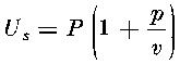[6], where

is the daily precession of the orbital plane,

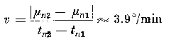is the average angular velocity easily measurable on the observed path elements. The sidereal period proved to be longer than the nodal one by 3-4 sec. Consequently satellite accelerations as derived refer practically to a perigee altitude of 255 km. CONCLUSIONS The Interobs program sets as an aim the investigation of sudden changes in the upper atmosphere as revealed by satellite drag. Studying the observational data on 1960 epsilon3 (1960 05/3) we demonstrated the possibility of regarding dP/dn as constant for time intervals of 8-10 days (at least during and about the minimum of solar activity) and to derive its mean value with no more than 20% external relative error. Consequently the density of the atmosphere near the perigee altitude of the satellite proved to be constant during most of the time intervals under consideration. Nevertheless we did not intend to determine it numerically for the following reasons: we did not succeed to derive the argument of perigee (the observations covering only a small fraction of the whole orbit) and also the effective cross-sectional area of the satellite is unknown. As the possibility of a slow precessional motion of the axis of rotation of the satellite (with a period of rotation of the order of weeks !) cannot be precluded [13], absolute measurements of air density are hampered by the corresponding variations of the cross-sectional area of the satellite at least if only one satellite is under observation. Sudden variations, like the one shown on Fig. 2 and 3, however, cannot be regarded as anything else but as the consequences of sudden changes in the density of the upper atmosphere. Hence according to the changes of drag acting on 1960 epsilon3, air density near its perigee altitude decreased by 31% on the 26^th August 1963. The change exceeds six times the standard error of dP/dn for the preceding time interval. It is natural to try to find a connection between this density decrease and variations in the actual solar activity, because a strong correlation between certain solar phenomena and the upper atmosphere is well known [14]. Exactly on the day mentioned a larger sunspot group turned away to the farside of the Sun, and, as a result, the Wolf (sunspot) number (R) dropped to about one half of its previous level. At the same time according to Catanian measurements the spot area (A) decreased to less than one third [15]. The coincidence of the solar and upper atmospheric events is interesting (see Fig. 3). Significant flares or distinctive events have not been observed during the time interval under consideration. In 1964 solar activity had reached its absolute minimum, the average sunspot number being only 4 in April and July, 5 in September [15]. There were no visible spots on the Sun during 7-12 July and 16-28 Sept; average sunspot numbers being as low as 7-8-9 in April. It is by no means surprizing that the acceleration dP/dn proved to be constant during these time intervals, and its absolute value in April 1964 was considerably larger than in July or in September. The correlation "more intensive solar activity - more intensive drag" approximately holds true, suggesting that with decrease in solar activity the upper atmosphere becomes cooler and shrinks closer to the earth so that at a given geometric altitude the density becomes less. The comparison of dP/dn values obtained for different time intervals demands, however, a lot of precaution because of the shift of the perigee and changes of the effective cross-sectional area as mentioned above. The general tendency - i.e. that a cceleration contrary to all expectations is a decreasing function of time - has been proved by the convex shape (as seen from below) of the

plot independently. From the graphically derived slopes of the curve at different points we find |dP/dn|^* decreasing as well (seeTable 5); even the arithmetical means of the (dp/dn)^* and dP/dn values derived during the four time intervals under consideration are practically equal (-0.00839 and -0.00861 s/rev respectively). Accordingly our results suggest that during 1963/64 air density around the altitude 250-260 km decreased - parallel with solar activity - to such an extent that the drag encountered by satellite 1960 epsilon3 did not show a rising but a falling tendency considerably prolonging the lifetime of the satellite. It would be an interesting task to determine whether similar effects occurred in the motion of other satellites at the same time; unfortunately the Interobs material available did not allow such an investigation. Studying all observations of 1960 epsilon3 in 1963/64 it could be ascertained that in time intervals when at least 3 transits have been well observed (simultaneously from two stations), the rate of change of the period of revolution, if constant, can be determined with an error not exceeding 10-15%. Supposing that sudden variations occur in air density which has an effect on dP/dn larger than this value, the date of change can be computed with an accuracy of possibly less than one day (in a fortunate case) or at least 1-2 days. Such time resolution is of interest when investigating the time delay of the influence of certain solar phenomena upon the upper atmosphere. It seems useful to extend the Interobs program in order to obtain material rich enough to set up actual correlations. Konkoly Observatory, Budapest, September 1965. APPENDIX PROGRAM FOR ELLIOTT 803 COMPUTER TO CALCULATE THE SATELLITE'S POSITION IN SPACE FROM SIMULTANEOUS OBSERVATIONS This program forms only the first part of a larger one to evaluate orbital elements directly from simultaneous observations (see [9]). The output of some data in excess is needed for the second part. Input data No. 1. number of tracking stations (less than 40); No. 2. coordinates of tracking stations in a rectangular and in a geographic system:

No. 3. number of days when observations have been performed (less than 200); No. 4. hours, minutes and seconds of Greenwich sidereal time at 0^h GMT of days when observations have been performed; No. 5. A_1 and A_2 (Parameters in

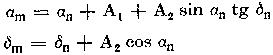where m is the year of observation, n is the epoch of the catalogue or atlas); No. 6. year, month, day and hour (integer numbers) of the first transit; No. 7. identification number of the satellite (integer of maximum 5 figures); No. 8. observing data: weight, time (h, m, s), identification number of the coordinate system (1 means equatorial, 2 means horizontal), right ascension or azimuth (h, m, s or °, ', ") declination or elevation (°,') serial number of the tracking station according to No. 2, and serial number of the day according to No. 4. N.B. Maximum number of simultaneity groups (points in space) on each transit is 100. More than one observation from the same tracking station cannot be used in one simultaneity group. Arriving to the next transit write all input data (No. 8) of the first observation, then 38( 40( and the time of the new transit as in No. 6. In the case of a new satellite add 39( and the identification number of the satellite as in No. 7. After the very last observation add 12 zeros and 38( 34( ). Output Every transit is printed out as a separate group. The first line gives: 1. the identification number of the satellite, 2. year, month, day and hour of the transit. Line No. 2: time (in degrees) and Theta (in degrees, see [9])of the first real observation; Line No. 3:

for the given transit. Spatial coordinates are tabulated below as follows:

where n_i is the number of all possible pairs in the simultaneity group when determining the satellite's position in space. The sign 5( at the end of every transit belongs to Part II. of the program. After the last transit all observations neglected during the calculation are printed out using the following code: Starting from horizontal coordinates

starting from equatorial coordinates

Numbers after these six-figure symbols give the serial number of the observation under consideration. Further, whilst determining a position in space, those pairs of observations are not used where

these are indicated by the symbol 666666 and k and l are printed out afterwards. SETS LIHJUVKQWCD(2002)E(4) VARY I=1:1:9 SETV P(240)A(205)B(23)S(160)G(10) READ B(I) N(11)Z(400) REPEAT I SETF TRIG ARCTAN SQRT READ Q SETR 40 READ W JUMP IF J=1TO20 1) READ L JUMP UNLESS B3=B13TO3 VARY I=I : 1 : L JUMP UNLESS B2=B12TO3 VARY H=0 : 40: 6 JUMP UNLESS B1=B11TO3 READ P(I+H) JUMP TO5 REPEAT H 20) B11=B1 REPEAT I B12=B2 READ L B13=B3 VARY I=1 :1:L B3=.01666666 * B3 READ A(I) B2=B2+B3 READ A(I+1) B2=.01666666 * B2 READ A(I+2) B1=B1+B2 A(1+2)=.01666666 * A(I+2) B20=15*B1 A(I+1)=A(I+2)+A(I+1) B1=1.00273791 * B20 A(I+1)=.01666666 * A(I+1) B14=B1+A(W) A(I)=A(I)+A(I+1) 23) JUMP UNLESS B14> 360TO4 A(I)=15 * A(I) B14=B14-360 REPEAT I JUMP TO23 READ G9 4) B1=B14/180 READ G10 B15=SIN B1 N1=0 B16=COS B1 N4=0 5) B1=P(Q) * B16 N8=0 B2=P(Q+40) * B15 VARY I=I :1:4 S(J+4)=B1-B2 READ EI B1=P(Q) * B15 REPEAT I B2=P(Q+40) * B16 2) READ V S(J+5)=B1+B2 C=1001 S(J+6)=P(Q+80) H=0 JUMP IF B4=1TO16 21) D2001=0 JUMP IF B8>60TO10 J=1 JUMP IF B8> 30TO9 U=0 JUMP IF B8>20TO8 22) READ S(J) JUMP IF B8> 15TO7 JUMP IF B8> 12TO6 12) B1=B14-B7 B9=B9-5 B1=B1-P(Q+120) JUMP TO10 26) JUMP IF B1 <0TO14 6) B9=B9-4 13) JUMP IF B1 < 360TO15 JUMP TO10 B1=B1-360 7) B9=B9-3 JUMP TO13 JUMP TO10 14) B1=B1+360 8) B9=B9-2 JUMP TO26 JUMP TO10 15) 131=131/180 9) B9=B9-1 B2=SIN B1 10) B7=.01666666 * B7 B3=MOD B2 B6=B7+B6 JUMP UNLESS B3>.99996TO27 B6=.01666666 * B6 D(C)=333333 B5=B5+B6 C=C+1 B9=.01666666 * B9 U=U+1 B8=B9+BS D(C)=U B5=B5/180 C=C+1 B6=COS B5 JUMP IF C> 1997TO34 B5=SIN B5 JUMP TO22 B8=B8/180 27) B1=COS B1 B9=COS B8 S(J+1)=B2/B1 B8=SIN B8 S(J+7) =8 (J+4)*(J+1) B1=P(Q+160) * B8 S(J+2)=1/B1 B2=P(Q+200) * B9 JUMP TO19 B2=B2*B6 16) B7=.01666666*B7 B1=B1+B2 B6=B6+B7 JUMP UNLESS B1 > .999TO24 B6=.01666666*B6 D(C)=111111 B5=B5+B6 C=C+1 B5=15*B5 U=U+1 B9=.01666666*B9 D(C)=U B8=B8+B9 C=C+1 B7=B5/180 JUMP IF C> 1997TO34 B6=COS B7 JUMP TO22 B7=SIN B7 24) B2=B1*B1 B7=G10*B7 B2=1-B2 B6=G10*B6 B2=SQRT B2 B9=B8/180 S(J+3)=B1/B2 B9=TAN B9 B3=-B9*B5 B7=B7*B9 B2=B3/B2 B7=B7+G9 B3=MOD B2 B5=B5+B7 JUMP UNLESS B3>.99996TO25 B8=B8+B6 D(C)=222222 JUMP IF BS < 90TO17 C=C+1 B8=180-B8 U=U+1 B5= B5+ 180 D(C)=U 17) JUMP UNLESS B8>87.5TO28 C=C+1 D(C)=444444 JUMP IF C> 1997TO34 C=C+1 JUMP TO22 U=U+1 25) B3=P(Q+160) * B1 D(C)=U B3=B8-B3 C=C+1 B7=B2*B2 JUMP IF C> 1997TO34 B7=1-B7 JUMP TO 22 B7=SQRT B7 28) JUMP UNLESS B5<0TO29 B7=B2/B7 B5=360+B5 B7=ARCTAN B7 JUMP TO28 B7=180 * B7 29) JUMP IF B5 < 360TO18 JUMP IF B2 > 0TO11 B5=B5-360 JUMP IF B3> 0TO 12 JUMP TO29 B7=-180-B7 18) 138=138/180 JUMP TO12 S(J+3)=TAN B8 11) JUMP IF B3 > 0TO 12 B5=B5/180 B7=180-B7 B2=SIN B5 B8=MOD B2 G2=G2+S(K+6) JUMP UNLESS B8>.99996TO30 G4=8(K)*G2 D(C)=555555 N3=N3+G4 C=C+1 G1=G1-S(L+4) U=U+1 G1=G1*S(L+3) D(C)=U G1=G1*S(L+2) C=C+1 G1=S(L+6)+G1 JUMP IF C> 1997TO34 G1=G1*S(L) JUMP TO 22 N3=N3+G1 30) 135=COS B5 I=I+1 S(J+1)=B2/B5 35) L=L+8 S(J+7)=S(J+4)*S(J+1) JUMP IF L <JTO31 S(J+2)=1/B5 33) K=K+8 19) U=U+1 L=K+8 D2001=D2001+ 1 JUMP IF L < JTO31 JUMP UNLESS D2001=1TO37 D(H)=I B22=1320 Z(4H+1)=N7/N5 B23=1314 Z(4H+2)=N2/N5 37) J=J+8 Z(4H+3)=N3/N6 JUMP TO22 B17=Z(4H+1)*Z(4H+1) 3) I=0 N1=N1+B17 N2=0 B18=Z(4H+2)*Z(4H+2) N3=0 N4=N4+B18 N5=0 B19=Z(4H+3)*Z(4H+3) N6=0 N8=N8+B19 N7=0 B17=B17+B18 K=1 B17=B17+B19 L=K+8 Z(4H+4)=SQRT B17 31) G7=8(K)*S(L) H=H+1 N5=N5+G7 S1=S J G8=S(K)+S(L) J=1 N6=N6+G8 JUMP TO20 G1=S(L+5)-S(K+5) 38) LINE G1=G1-S(L+7) PRINT V,5 G1=G1+S(K+7) SPACES 5 G2=S(K+ 1)-S(L+ 1) PRINT E1,4 G6=MOD G2 PRINT E2,2 JUMP UNLESS G6<.1TO32 PRINT E3,2 D(C)=666666 PRINT E4,2 C=C+1 LINE D(C)=K PRINT B22 C=C+1 PRINT B23 D(C)=L LINE C=C+1 PRINT N1 JUMP UNLESS C > 1997TO35 PRINT N4 LINE PRINT N8 D2002 =C-1001 LINE VARY C=1001 : 1 : D2002 VARY I=0 : 1 : H PRINT D(C) VARY K=1 : 1 : 4 LINE PRINT Z(4I+K) REPEAT C REPEAT K C=1001 PRINT DI JUMP TO35 LINE 32) G1=G1/G2 REPEAT T G6=G1*G7 OUTPUT 21 N7=N7+G6 OUTPUT 17 G2=G1-S(K+4) N1=0 G3=G2*S(K+1) N4=0 G3=S(K+5)+G3 N8=0 G5=G3*G7 D2001=0 N2=N2+G5 H=0 G2=G2*S(K+3) JUMP TO22 G2=G2*S(K+2) 34) C=C-1 LINES 3 JUMP TO22 CYCLE K=1001 : 1: C 40) VARY I=1 : 1: 4 PRINT DK,6 READ EI LINE REPEAT I REPEAT K JUMP TO22 C=1001 36) STOP JUMP TO22 START 1 39) READ V REFERENCES [1] D. G. King-Hele and D. M. C. Walker: Space Research 2, p. 918, 1961. D. G. King-Hele: JBIS 19, p. 374, 1964. R. H. Merson and A. T. Sinclair: RAE Technical Rep. No 64036, 1964. M. Ill: Nabljudenija ISZ 3, 1964. M. J. Marov: Kosmiceskie issledovania Vip 6 1964. [2] e.g. H. F. Michielson: PhS and E 6 No 6 1962. [3] Z. Ceplecha: BAC 10 41 1958. C. Popovici: Nabljudenija ISZ 1 33 1962. [4] D. E. Segolev Nabljudenija ISZ 1 40 1962. [5] G. Veis: SAO Sp. Rep. No 133 1962. [6] M. Ill: Baja Mitt. No. 1 1962. [7] Ergebnisse der im Rahmen des Interobs-Programms abgehaltenen Kooperationswochen 1, 2, 1964, 1965. [8] J. Bienewski: Biuletyn polskich ... 8 58 1963. W. Baran: Artificial Earth Satellites. Observations and Investigations in Poland 105 1965. I. Almár and M. Ill: Nabljudenija ISZ 1 46 1962. [9] E. Illés and I. Almár: Nabljudenij ISZ 3 1964. [10] G. A. Ustinov: Nabljudenija ISZ 2 19 1963 [11] e.g. D. G. King-Hele: Progress in the Astronautical Sciences 1 1962. (The same equation used with two different coefficients.) [12] G. A. Cebotarev - E. N. Makarova: Bjulleteni stancii ... No 40 34 1964. [13] L. G. Jacchia: Smithsonian Astrophysical Observatory 1962 Dez 31. [14] e.g. H. K. Paetzold and H. Zschörner: Space Research 1 p. 28 1960. N. L. Slovohotova: Nabljudenia Isz 2 3 1963. [15] Quarterly Bulletin on Solar Activity, Eidgen Sternwarte Zürich Solnecnije dannie ERRATA In Mitteilunlgen der Sternwarte der Ungarischen Akademie der Wissenschaften Nr. 59 p. 9 last two equations read