Non-Periodic Phenomena in Variable Stars
IAU Colloquium, Budapest, 1968
COOPERATIVE 24-HOUR OBSERVATIONS OF UV CETI-TYPE STARS
P. F. CHUGAINOV
Crimean Astrophysical Observatory, USSR
Since 1967 the Working Group on UV Cet-type stars has organized and
carried out runs of 24-hour photometric observations of these stars. Our
aim is to study the time distribution of flares.
The following observers took part in the observations:
Australia: members of the Astronomical Society of N.S.W., coordinators
C. S. Higgins and G. E. Patston.
Italy: Catania Observatory, G. Godoli.
Japan: Tokyo Astronomical Observatory, K. Osawa et al.
New Zealand: Mt. John Observatory and amateur astronomers, coordinator
F. M. Bateson.
South Africa: Boyden Observatory, J. P. Eksteen.
U.S.A.: Smithsonian Astrophysical Observatory, L. H. Solomon. Steward
Observatory, B. Westerlund.
U.S.S.R.: Abastumani Astrophysical Observatory, V. S. Oskanjan. Crimean
Astrophysical Observatory P. F. Chugainov.
At present, several other observatories have agreed to take part in
future programmes.
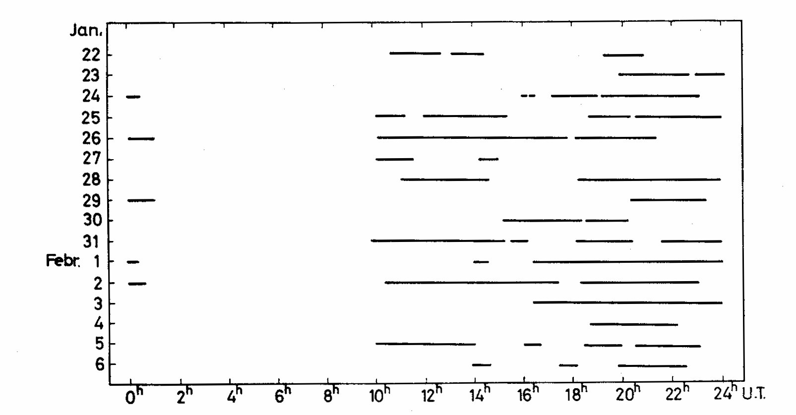 Fig. 1. Time coverage of the material on YZ CMi
Up to now two observational campaigns have been carried out: September
26-October 10, 1967, UV Cet and January 22-February 6, 1968, YZ CMi.
During the first period 50.5 per cent of total time was covered by
observations. 17.9 per cent being photoelectric and 32.6 per cent
photographic and visual observations. Only photoelectric observations
were made during the second period, the coverage being 29.5 per cent of
the total time.
Most of the observational results have been published in I.B.V.S.
(1968). The study of the time distribution of flares has been carried
out by K. Osawa et al. (1968). At the Crimean Astrophysical Observatory
A. A. Korovyakovskaya and the Author have analyzed the observations from
both periods. Now we have completed the study of the material on YZ CMi.
We used the autocorrelation analysis in order to study the time
distribution of flares. The observational period was divided into equal
time intervals tau. tau = 30 minutes was adopted. For the periods of 15 days
the total number of time intervals was equal to 720. Energies I emitted
for each interval were computed according to observational data. One can
see that I = I_norm if the flares are absent, and I = I_norm + I_flare in
the presence of a flare, I_norm, I_flare being the integrated energies
emitted by the star and flare, respectively. For each time interval i,
the quantity
u_i=I_i-mean(I)
was determined where
mean(I)=Summa(I_i)/N.
Autocorrelation functions
Fig. 1. Time coverage of the material on YZ CMi
Up to now two observational campaigns have been carried out: September
26-October 10, 1967, UV Cet and January 22-February 6, 1968, YZ CMi.
During the first period 50.5 per cent of total time was covered by
observations. 17.9 per cent being photoelectric and 32.6 per cent
photographic and visual observations. Only photoelectric observations
were made during the second period, the coverage being 29.5 per cent of
the total time.
Most of the observational results have been published in I.B.V.S.
(1968). The study of the time distribution of flares has been carried
out by K. Osawa et al. (1968). At the Crimean Astrophysical Observatory
A. A. Korovyakovskaya and the Author have analyzed the observations from
both periods. Now we have completed the study of the material on YZ CMi.
We used the autocorrelation analysis in order to study the time
distribution of flares. The observational period was divided into equal
time intervals tau. tau = 30 minutes was adopted. For the periods of 15 days
the total number of time intervals was equal to 720. Energies I emitted
for each interval were computed according to observational data. One can
see that I = I_norm if the flares are absent, and I = I_norm + I_flare in
the presence of a flare, I_norm, I_flare being the integrated energies
emitted by the star and flare, respectively. For each time interval i,
the quantity
u_i=I_i-mean(I)
was determined where
mean(I)=Summa(I_i)/N.
Autocorrelation functions
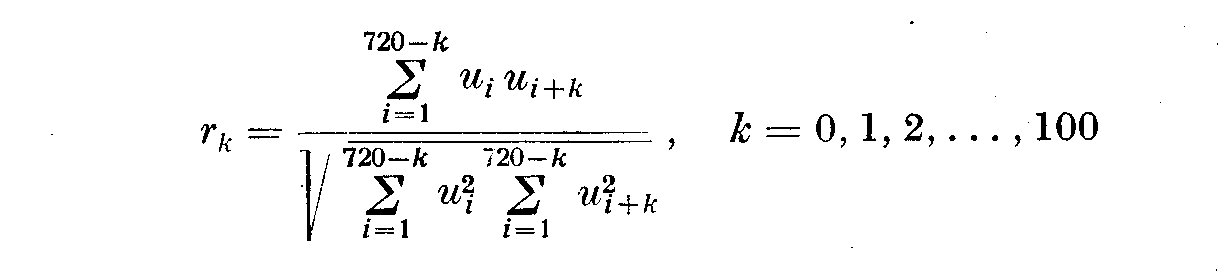 were computed, using u_i for those time intervals which had been covered
by observations. The computations were carried out with an electronic
computer Minsk-1. Earlier, such method was used by Lukatskaya (1967) for
the analysis of light curves of irregular variables of RW Aur and U
Gem-type.
The variation of r_k with k is shown in Fig. 2. The obtained curve
differs from that which could be expected in the case of Poisson's
distribution of flares in time. Therefore, it gives rather good evidence
of periodicity of flares. On the curve, there are six maxima repeating
almost periodically, the period being about 14 tau, i.e. 7 hours.
We have tried different elements in order to represent the times of
observed flares. The following elements have been found to be the best
ones:
Time of max. (UT) = Jan. 23 (1968), 2 + 6h50m24s X E.
The representation obtained is shown in Table 1. It is seen that in
several cases two or even three flares were observed near the times
given by the elements. In such cases, if the energies of flares are
nearly equal, the mean time of maxima was adopted as the observed time.
If the energy of one flare of the
Table 1. Flares of YZ CMi
Observer Time of max. Integral energy O-C
of flare, U. T. of flare, minutes
Eksteen Jan. 23, 21h29.6m 19.2
0h00m
22h09.0m 1.3
23h23.6m 0.4
Osawa et al. Jan. 24, 17h22.5m 0.35
17h34.2m 0.25
17h56.7m 3.5 -0h04m
Osawa et al. Jan. 25, 12h53.2m 0.7 -1h13m
13h42.7m 0.25
Oskanjan Jan. 26, 19h17.0m 1.5 +1h24m
Eksteen Jan. 29, 0h29.7m 1.4 -0h07m
Eksteen Jan. 29, 20h29.7m 1.4
21h39.7m 14.0 +0h32m
Osawa et al. Jan. 31, 12h23.4m 0.3 -1h36m
12h45.5m 0.3
Chugainov Jan. 31, 19h58.0m 0.23 -1h03m
Chugianov Feb. 1, 18h21.0m 0.32 +0h49m
Osawa et al. Feb. 2, 15h58.9m 0.15 +1h55m
Eksteen Feb. 2, 19h14.3m 0.6 -1h41m
Chugainov Feb. 3, 22h49.0m 0.68 -1h26m
Oskanjan Feb. 4, 20h36.2m 5.0
21h13.4m 15.0 -0h26m
Osawa et al. Feb. 5, 10h45.0m 7.0 -0h35m
11h20.0m 5.0
12h14.9m 0.35
group is essentially greater than that of the others, then O-C was
computed only for this flare and the others were neglected. The mean O-C
was obtained to be 1h 06m. The tendency of flares to form groups was
noticed by Osawa et al. (1968).
were computed, using u_i for those time intervals which had been covered
by observations. The computations were carried out with an electronic
computer Minsk-1. Earlier, such method was used by Lukatskaya (1967) for
the analysis of light curves of irregular variables of RW Aur and U
Gem-type.
The variation of r_k with k is shown in Fig. 2. The obtained curve
differs from that which could be expected in the case of Poisson's
distribution of flares in time. Therefore, it gives rather good evidence
of periodicity of flares. On the curve, there are six maxima repeating
almost periodically, the period being about 14 tau, i.e. 7 hours.
We have tried different elements in order to represent the times of
observed flares. The following elements have been found to be the best
ones:
Time of max. (UT) = Jan. 23 (1968), 2 + 6h50m24s X E.
The representation obtained is shown in Table 1. It is seen that in
several cases two or even three flares were observed near the times
given by the elements. In such cases, if the energies of flares are
nearly equal, the mean time of maxima was adopted as the observed time.
If the energy of one flare of the
Table 1. Flares of YZ CMi
Observer Time of max. Integral energy O-C
of flare, U. T. of flare, minutes
Eksteen Jan. 23, 21h29.6m 19.2
0h00m
22h09.0m 1.3
23h23.6m 0.4
Osawa et al. Jan. 24, 17h22.5m 0.35
17h34.2m 0.25
17h56.7m 3.5 -0h04m
Osawa et al. Jan. 25, 12h53.2m 0.7 -1h13m
13h42.7m 0.25
Oskanjan Jan. 26, 19h17.0m 1.5 +1h24m
Eksteen Jan. 29, 0h29.7m 1.4 -0h07m
Eksteen Jan. 29, 20h29.7m 1.4
21h39.7m 14.0 +0h32m
Osawa et al. Jan. 31, 12h23.4m 0.3 -1h36m
12h45.5m 0.3
Chugainov Jan. 31, 19h58.0m 0.23 -1h03m
Chugianov Feb. 1, 18h21.0m 0.32 +0h49m
Osawa et al. Feb. 2, 15h58.9m 0.15 +1h55m
Eksteen Feb. 2, 19h14.3m 0.6 -1h41m
Chugainov Feb. 3, 22h49.0m 0.68 -1h26m
Oskanjan Feb. 4, 20h36.2m 5.0
21h13.4m 15.0 -0h26m
Osawa et al. Feb. 5, 10h45.0m 7.0 -0h35m
11h20.0m 5.0
12h14.9m 0.35
group is essentially greater than that of the others, then O-C was
computed only for this flare and the others were neglected. The mean O-C
was obtained to be 1h 06m. The tendency of flares to form groups was
noticed by Osawa et al. (1968).
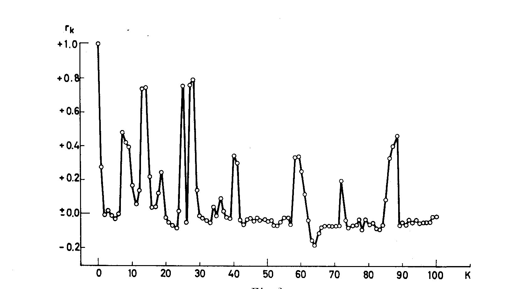 Fig. 2.
The period of repetition of flares was found to be 20.2h by Osawa et al.
(1968). Andrews (1966) found from observations of YZ CMi in 1966 that
the intervals between flares were equal to 47h, 73h or 122h. These data
do not contradict our result because 6h50m24s X 3 = 20.5h, 6h50m24s X 7
= 47.9h, 6h50m24s X 11 = 75.2h and 6h50m24s X 18 = 123.1h. It is obvious
that Andrews and Osawa have found periods which are divisible by our
period. Our result shows the importance of making observations at
several observatories located at different longitudes.
We have tried to represent the times of flares of YZ CMi observed by
Andrews in 1966. It was found that the elements:
Time of max (UT) = Feb. 21 (1966), 18h 32m + 6h 38.9m X E, represent all
the flares observed, with a mean deviation of 1h 22m.
REFERENCES
Andrews, A. D., 1966, Publ. astron. Soc. Pacific 78, 324.
Information Bulletin on Variable Stars nos. 264, 265, 267, 268. 1968.
(IBVS N°.264)
(IBVS N°.265)
(IBVS N°.267)
(IBVS N°.268)
Lukatskaya, F. I., 1967, Perem. Zvezdy, 16, 168.
Osawa, K., Ichimura, K., Noguchi, T., and Watanabe, E., 1968, Tokyo astr. Bull.,
Second Series no. 180.
Fig. 2.
The period of repetition of flares was found to be 20.2h by Osawa et al.
(1968). Andrews (1966) found from observations of YZ CMi in 1966 that
the intervals between flares were equal to 47h, 73h or 122h. These data
do not contradict our result because 6h50m24s X 3 = 20.5h, 6h50m24s X 7
= 47.9h, 6h50m24s X 11 = 75.2h and 6h50m24s X 18 = 123.1h. It is obvious
that Andrews and Osawa have found periods which are divisible by our
period. Our result shows the importance of making observations at
several observatories located at different longitudes.
We have tried to represent the times of flares of YZ CMi observed by
Andrews in 1966. It was found that the elements:
Time of max (UT) = Feb. 21 (1966), 18h 32m + 6h 38.9m X E, represent all
the flares observed, with a mean deviation of 1h 22m.
REFERENCES
Andrews, A. D., 1966, Publ. astron. Soc. Pacific 78, 324.
Information Bulletin on Variable Stars nos. 264, 265, 267, 268. 1968.
(IBVS N°.264)
(IBVS N°.265)
(IBVS N°.267)
(IBVS N°.268)
Lukatskaya, F. I., 1967, Perem. Zvezdy, 16, 168.
Osawa, K., Ichimura, K., Noguchi, T., and Watanabe, E., 1968, Tokyo astr. Bull.,
Second Series no. 180.