Non-Periodic Phenomena in Variable Stars
IAU Colloquium, Budapest, 1968
THE CLASSIFICATION OF PHOTOMETRIC
LIGHT-CURVES OF FLARES OF UV CETI STARS
V. S. OSKANIAN
Byurakan Astrophysical Observatory, Armenia, USSR
One of the means to investigate the flare phenomenon of the UV Ceti
stars is to study its photometric light-curve characteristics, for it
can be supposed that in principle the form of the light-curve depends on
the type of process taking place on the star. Such studies have already
been made (Chugainov, 1962; Oskanian, 1957; Roques, 1961). It is
noteworthy, that all of them were not dealing with the light-curve as a
whole but with its decreasing branch only. Moreover, the number of
curves studied in this way has been very limited.
The number of precise photoelectric observations increased significantly
during the last few years resulting in the discovery of a great variety
of forms of flare light-curves. This fact called for a rather different
approach to the study of light-curves. (An example of such a new
approach is W. Kunkel's (1967) attempt to treat the curves as composed
from two - slow and fast - superposed components). Now it seems more
correct to substitute the detailed study of single curves by a
classification of them, based on such parameters which can be determined
for all kinds of flare curves. In this case, the study of details of
light-curves should be renounced as it can be supposed that their
general features are more substantial than the small amplitude details.
The aim of the present paper is to propose one of the possible kinds of
classification of flare light-curves. The proposed classification is
based on the following two parameters of the light-curve:
a) the rate of brightness-increase;
b) the character of the decreasing branch of the light-curve.
Four types of photometric light-curves can be defined by means of these
two parameters. Two of them may be considered as extremal in the sense
that they possess extremal values of the parameter "a" and substantially
different parameters "b", while the other two types should be regarded
as intermediate.
These four types of flare light-curves could be denoted by I, II, III,
IV and defined as follows:*
* A third parameter t/T (t the time of rise from normal state to maximum
and T the duration of the whole flare) could be used as well, but it
seems that it is less precise than the proposed two parameters for the
following reasons:
1. It is difficult to determine the precise moment of ending of the
flare, i.e. the right value of T.
2. A prolonged "tail" of the flare, that appears sometimes, can make
this parameter rather indefinite.
Nevertheless, it is quite obvious that on the average the value of this
parameter should increase with the increasing number of curve types,
attaining a value of about 0.5 for Type IV curves.
Type I. This type is characterized by a great rate of brightness-increase
(in the studied cases this rate was between 5 and 1 magnitudes per
minute). The brightness-decrease starts immediately after the maximum
and takes place with the same rapidity as the increase, producing thus a
very sharp maximum. The rate of decrease slows down only in the final
phase of the flare. In the stellar magnitude scale the decreasing branch
of the curve can be approximated by two straight lines. In other words,
if one tries to represent the decreasing branch - expressed in intensity
scale - by the formula
I = IM e^-alpha(t-tM), (1)
it would be necessary to choose two different values of alpha in order to
approximate the curve of this type (Chugainov, 1962).
Examples of Type I curves are given on Fig. 1.
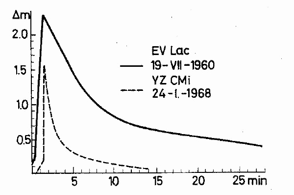 Fig. 1
Type IV. Being the other extremal case, this type of curves is characterized
by a very small rate of brightness-increase (not greater than some tenths of
magnitude per minute), a flat maximum and a small rate of brightness-decrease.
In the stellar magnitude scale the decreasing branch can be approximated by a
single straight line. The approximation by formula (1) can be realized by using
a single value of alpha.
Examples of Type IV curves are given on Fig. 2.
Fig. 1
Type IV. Being the other extremal case, this type of curves is characterized
by a very small rate of brightness-increase (not greater than some tenths of
magnitude per minute), a flat maximum and a small rate of brightness-decrease.
In the stellar magnitude scale the decreasing branch can be approximated by a
single straight line. The approximation by formula (1) can be realized by using
a single value of alpha.
Examples of Type IV curves are given on Fig. 2.
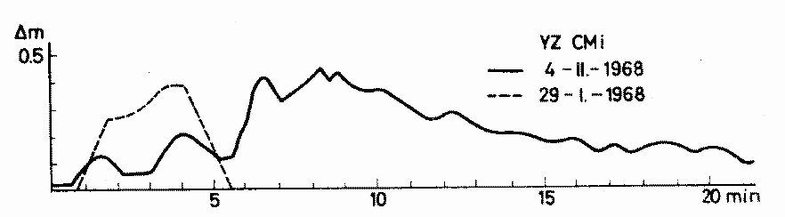 Fig. 2
Type II. The curves of this type seem to be composed of curves of Types
I and IV, the first part of the curve having Type I and the second part
Type IV characteristics. The transition from Type I to Type IV is very
rapid and takes place at different phases of the decreasing branch.
Examples of Type II curves are given on Fig. 3.
Fig. 2
Type II. The curves of this type seem to be composed of curves of Types
I and IV, the first part of the curve having Type I and the second part
Type IV characteristics. The transition from Type I to Type IV is very
rapid and takes place at different phases of the decreasing branch.
Examples of Type II curves are given on Fig. 3.
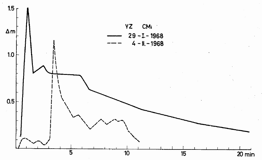 Fig. 3
Type III. By its appearance - especially by its relatively sharp maximum - the
curves of this type are very similar to those of Type I, but they differ from
the last ones by their smaller rate of brightness-increase (nearly always
smaller than one magnitude per minute). In the stellar magnitude scale the
decreasing branch can be approximated by a single straight line, i.e., by
one value of alpha in formula 1.
Examples of Type III curves are given on Fig. 4.
Fig. 3
Type III. By its appearance - especially by its relatively sharp maximum - the
curves of this type are very similar to those of Type I, but they differ from
the last ones by their smaller rate of brightness-increase (nearly always
smaller than one magnitude per minute). In the stellar magnitude scale the
decreasing branch can be approximated by a single straight line, i.e., by
one value of alpha in formula 1.
Examples of Type III curves are given on Fig. 4.
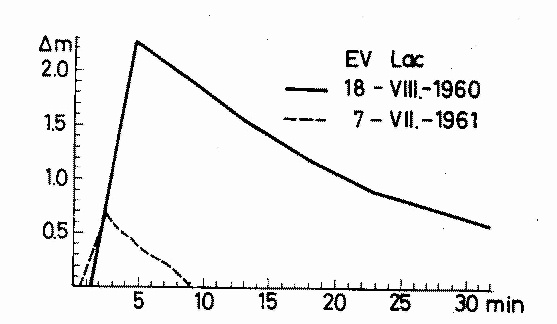 Fig. 4
A list of 30 flares classified by means of the two mentioned parameters is
given in Table I. It should be noted that the accuracy of data used to prepare
this Table was not sufficiently homogeneous, so that some unessential
changes - especially in the values of Delta m/Delta t - could be allowed.
The uncertainty in the classification of flare No. 21 should also be ascribed
to the impossibility of getting more accurate data from the published curves.
Table I
A = No.
B = Delta m / Delta t
C = Type
D = Delta m_B
E = Star
F = Date
G = Author
A B C D E F G
1 5.2 I 1.56 YZ CMi 24. I. 1968 Osawa et al.
2 5.1 I 1.52 UV Cet 26. IX. 1965 Chugainov
3 4.9 I 1.23 EV Lac 21. IX. 1960 Chugainov
4 4.8 II 1.12 YZ CMi 4. II. 1968 Oskanian
5 3.0 II 1.51 YZ CMi 29. I. 1968 Eksteen
6 3.0 I 0.90 EV Lac 21. IX. 1960 Chugainov
7 2.9 I 2.88 EV Lac 27. VIII. 1962 Chugainov
8 2.6 I 1.32 YZ CMi 5. II. 1968 Osawa et al.
9 2.3 I 2.29 EV Lac 19. VII. 1960 Chugainov
10 2.2 I 1.10 UV Cet 20. IX. 1965 Chugainov
11 1.8 I 1.90 UV Cet 24. IX. 1965 Chugainov
12 1.8 II 1.83 YZ CMi 23. I. 1968 Eksteen
13 1.8 I 0.54 EV Lac 4. X. 1961 Chugainov
14 1.5 II 0.81 EV Lac 14. IX. 1961 Chugainov
15 1.4 I 2.86 EV Lac 27. VIII. 1962 Chugainov
16 1.4 II 1.39 YZ CMi 5. II. 1968 Osawa et al.
17 1.3 I 1.52 EV Lac 31. VII. 1962 Chugainov
18 1.2 I 0.81 EV Lac 17. X. 1961 Chugainov
19 1.1 I 0.56 YZ CMi 1. III. 1968 Cristaldi
20 0.7 III 0.72 EV Lac 6. IX. 1961 Chugainov
21 0.6 III I 0.63 EV Lac 1. IX. 1961 Chugainov
22 0.6 III 0.36 YZ CMi 26. I. 1968 Oskanian
23 0.5 III 0.33 YZ CMi 23. II. 1968 Oskanian
24 0.5 III 2.30 EV Lac 18. VIII. 1960 Chugainov
25 0.4 III 0.70 EV Lac 7. VIII. 1961 Chugainov
26 0.4 III 0.75 V 1216 Sgr 28. VI. 1961 Grigorian,
Vardanian
27 0.2 III 3.21 YZ CMi 24. II. 1968 Oskanian
28 0.14 IV 0.39 YZ CMi 29. I. 1968 Eksteen
29 0.1 III 0.75 EV Lac 18. VIII. 1963 Chugainov
30 0.06 IV 0.46 YZ CMi 4. II. 1968 Oskanian
Nevertheless, the data listed in Table I allow the following qualitative
conclusions:
a) The rate of brightness-increase is greater than one magnitude per minute
for the curves of Type I and Type II, and less than this value for the curves
of Type III and Type IV.
b) There are some reasons to suppose that curves of Type IV appear
really more rarely than those of other types. As to the frequency
distribution of curves of different types (Table II) resulting from
Table I, it can not pretend to be a real one, owing to the sampling
effect caused by the suppression of a number of small amplitude flares.
Table II
Type Number of flares Mean values of Delta m_B
I 14 1.42
II 5 1.33
III 9 1.08
IV 2 0.43
c) There is no obvious correlation between the amplitude of light-variation
and curve-type. Nevertheless, it seems that the mean values of Delta m_B
for different types of curves show tendency to diminish from Type I to Type IV.
But, because of the above mentioned sampling effect, this conclusion too must
be accepted with some precaution.
It should be noted, at last, that in some rare cases the light-curve can
not be classified according to this classification. But in these cases too
the proposed classification does not lose its value, as the mentioned curves
are nearly always a combination of two or more curves of the types defined by
this classification.
So, for instance, the curve represented on Figure 5 can be interpreted
as a superposition of two Type I curves.
Fig. 4
A list of 30 flares classified by means of the two mentioned parameters is
given in Table I. It should be noted that the accuracy of data used to prepare
this Table was not sufficiently homogeneous, so that some unessential
changes - especially in the values of Delta m/Delta t - could be allowed.
The uncertainty in the classification of flare No. 21 should also be ascribed
to the impossibility of getting more accurate data from the published curves.
Table I
A = No.
B = Delta m / Delta t
C = Type
D = Delta m_B
E = Star
F = Date
G = Author
A B C D E F G
1 5.2 I 1.56 YZ CMi 24. I. 1968 Osawa et al.
2 5.1 I 1.52 UV Cet 26. IX. 1965 Chugainov
3 4.9 I 1.23 EV Lac 21. IX. 1960 Chugainov
4 4.8 II 1.12 YZ CMi 4. II. 1968 Oskanian
5 3.0 II 1.51 YZ CMi 29. I. 1968 Eksteen
6 3.0 I 0.90 EV Lac 21. IX. 1960 Chugainov
7 2.9 I 2.88 EV Lac 27. VIII. 1962 Chugainov
8 2.6 I 1.32 YZ CMi 5. II. 1968 Osawa et al.
9 2.3 I 2.29 EV Lac 19. VII. 1960 Chugainov
10 2.2 I 1.10 UV Cet 20. IX. 1965 Chugainov
11 1.8 I 1.90 UV Cet 24. IX. 1965 Chugainov
12 1.8 II 1.83 YZ CMi 23. I. 1968 Eksteen
13 1.8 I 0.54 EV Lac 4. X. 1961 Chugainov
14 1.5 II 0.81 EV Lac 14. IX. 1961 Chugainov
15 1.4 I 2.86 EV Lac 27. VIII. 1962 Chugainov
16 1.4 II 1.39 YZ CMi 5. II. 1968 Osawa et al.
17 1.3 I 1.52 EV Lac 31. VII. 1962 Chugainov
18 1.2 I 0.81 EV Lac 17. X. 1961 Chugainov
19 1.1 I 0.56 YZ CMi 1. III. 1968 Cristaldi
20 0.7 III 0.72 EV Lac 6. IX. 1961 Chugainov
21 0.6 III I 0.63 EV Lac 1. IX. 1961 Chugainov
22 0.6 III 0.36 YZ CMi 26. I. 1968 Oskanian
23 0.5 III 0.33 YZ CMi 23. II. 1968 Oskanian
24 0.5 III 2.30 EV Lac 18. VIII. 1960 Chugainov
25 0.4 III 0.70 EV Lac 7. VIII. 1961 Chugainov
26 0.4 III 0.75 V 1216 Sgr 28. VI. 1961 Grigorian,
Vardanian
27 0.2 III 3.21 YZ CMi 24. II. 1968 Oskanian
28 0.14 IV 0.39 YZ CMi 29. I. 1968 Eksteen
29 0.1 III 0.75 EV Lac 18. VIII. 1963 Chugainov
30 0.06 IV 0.46 YZ CMi 4. II. 1968 Oskanian
Nevertheless, the data listed in Table I allow the following qualitative
conclusions:
a) The rate of brightness-increase is greater than one magnitude per minute
for the curves of Type I and Type II, and less than this value for the curves
of Type III and Type IV.
b) There are some reasons to suppose that curves of Type IV appear
really more rarely than those of other types. As to the frequency
distribution of curves of different types (Table II) resulting from
Table I, it can not pretend to be a real one, owing to the sampling
effect caused by the suppression of a number of small amplitude flares.
Table II
Type Number of flares Mean values of Delta m_B
I 14 1.42
II 5 1.33
III 9 1.08
IV 2 0.43
c) There is no obvious correlation between the amplitude of light-variation
and curve-type. Nevertheless, it seems that the mean values of Delta m_B
for different types of curves show tendency to diminish from Type I to Type IV.
But, because of the above mentioned sampling effect, this conclusion too must
be accepted with some precaution.
It should be noted, at last, that in some rare cases the light-curve can
not be classified according to this classification. But in these cases too
the proposed classification does not lose its value, as the mentioned curves
are nearly always a combination of two or more curves of the types defined by
this classification.
So, for instance, the curve represented on Figure 5 can be interpreted
as a superposition of two Type I curves.
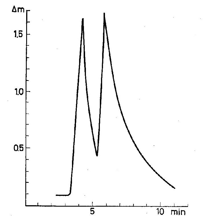 Fig. 5
REFERENCES
Chugainov, P. 1962. Izv. Krym. astr. Obs. XXVIII., 150.
Kunkel, W. 1967. Thesis, Univ. of Texas, Austin.
Oskanian, V. 1957. Nestacinarnie zvjozdi, Ac. Sc. of Armenia, Erevan.
Roques, P. 1961. Astrophys. J. 133, 914.
DISCUSSION
Godoli: Could it be possible, to approximate the decreasing part of your type
I flare light curves by an exponential function instead of two linear
functions?
Oskanian: In intensity scale you need two exponential functions, in stellar
magnitude scale two straight lines,
Fig. 5
REFERENCES
Chugainov, P. 1962. Izv. Krym. astr. Obs. XXVIII., 150.
Kunkel, W. 1967. Thesis, Univ. of Texas, Austin.
Oskanian, V. 1957. Nestacinarnie zvjozdi, Ac. Sc. of Armenia, Erevan.
Roques, P. 1961. Astrophys. J. 133, 914.
DISCUSSION
Godoli: Could it be possible, to approximate the decreasing part of your type
I flare light curves by an exponential function instead of two linear
functions?
Oskanian: In intensity scale you need two exponential functions, in stellar
magnitude scale two straight lines,