Non-Periodic Phenomena in Variable Stars
IAU Colloquium, Budapest, 1968
SPECTRAL ANALYSIS OF THE LIGHT CURVES OF T TAURI STARS
AND OTHER OBJECTS
STEPHEN PLAGEMANN
Institute of Theoretical Astronomy, Cambridge, England
LIST OF SYMBOLS
(1) f frequency in units of cycles per day.
(2) f_N Nyquist frequency, where fn = 1/2 Delta t
(3) omega angular frequency in radians, f_N = pi / Delta t
(4) Delta t sampling interval.
(5) n number of observations.
(6) lambda(k) lag of time domain window, also known as the covariance
averaging kernel.
(7) k number of lags in the time domain.
(8) m the total number of lags.
(9) X_i(t) observed time series (light curve).
(10) sigma^2 variance.
(11) mu_i mean of time series.
(12) gamma_11(k) sample estimate of the autocovariance of lag k uncorrected
for the mean.
(13) gamma_12(k) crosscovariance of X_1(t) and X_2(t).
(14) rho_11(k) autocorrelation coefficient.
(15) c_11(k) sample estimate of the autocovariance.
(16) r_12(k) ordinary product-moment correlation between X_1(t) and X_2(t).
(17) U_k series used as filter in time domain with convolution.
(18) T(omega) spectral window or kernel.
(19) b(omega) bias.
(20) nu degrees of freedom.
(21) B omega bandwidth.
(22) A_11(k) autocorrelation function of X_1(t).
(23) A_21(k) crosscorrelation function of X_2(t) and with X_1(t).
(24) I_11(omega) spectral estimate for harmonic analysis.
(25) eta(omega-y) spectral window in frequency domain.
(26) f (omega) spectral density function of X_1(t); the cosine transformation
of X_1(t).
(27) R_12 contribution to the sample variance from the jth harmonic.
(28) E(k) the energy per unit interval of f(a m Delta t) centred upon
k = 0, 1, ..., m.
(29) Z_(K) the co-spectrum; the cosine transformation of the crosscorrelation
(30) W(k) the quadratine spectrum; the sine transformation of the crosscorrelation.
(31) R(k) the coherence.
(32) theta(k) phase difference.
(33) G(omega) the gain.
(34) T(i omega) transfer function.
I. INTRODUCTION
The purpose of computing power spectra from the light curves of irregular
stars is both theoretical and practical. A power spectrum of a star is an
ideal method to study a complicated light or velocity curve whose inherent
periodicities may be obscured by noise. If one lacks theoretical light or
velocity curves, power spectrum analysis of the empirical data can reveal
the presence of peaks above the noise level, giving an exact value for the
periodicities and their amplitude, and the distribution of energy at different
vibrational frequencies. We can also study the changes in time of the period,
amplitude and energy distribution. This information can in turn be compared
with the T Tauri variables, such as their peculiar absorption and emission
spectra, their spectral type and their age and mass when compared to a
theoretical H-R diagram.
The preparation of power spectra of T Tauri stars involved a research scheme
carried out in three stages. Stage I began with an extensive search of the
literature over the past fifty years for published light curves of all the
130 T Tauri stars given in a table by Herbig (1962), plus some additions. This
task has been eased by references in two biographical works, "Geschichte und
Literatur des Lichtwechsels der Veränderlichen Sterne" and the "Astronomischer
Jahresbericht". It was necessary to check through each reference to discover
which contained the useful data. The light curves were then put on to punched
cards, each card having a single Julian Date and magnitude. After the light
curves were punched on IBM cards (some 27,000 readings in all) they were sorted
out serially and counted on an IBM 1401 computer, the light curves were printed
out and checked visually to reveal the presence of flares. The criteria used
was an increase in brightness greater than 0.4m in the course of one hour
passage. Stage II involved the calculation of pilot power spectra of T Tauri
stars for different sampling intervals Delta t and lags K in order to select
stable spectral estimates. Checks for stationarity and normality were made by
breaking up long data sequences in halves and comparing the power spectra of each.
Stage III of estimating the power spectra of T Tauri stars was done using
optimal sampling intervals and lags, i.e. those that all the essential details
appeared in the spectrum. An important factor in revealing the data was a
prewhitening or filtering of the data in order to reduce the effects of power
leakage from higher frequencies that tend to distort the power spectrum. As a
further check of the power spectrum's stability the light curves were converted
to a new time series by the addition of a Gaussian distributed random numbers
within a standard deviation of the mean, and the resulting power spectrum was
then computed. Definitions and procedural details will be presented below.
All of the computations involving time series used a system of programmes
(BOMM) developed by Bullard et al. (1966) for geophysical applications. The
calculations were carried out by the IBM 7090 computer at Imperial College,
London. Total computation times for each light curve analysed will be provided
and other details will be presented in a later paper.
II. TIME DOMAIN AUTOCORRELATION
In the following pages, two forms of spectral analysis will be discussed:
a) auto-spectral analysis of a single time series, and
b) cross-spectral analysis of pairs of time series for the purpose of
comparison of sets of empirical data with theoretical models.
We must first consider in the time domain some statistical limitations
upon the data. The spectrum of the discrete series X_1(t) is only defined
for frequencies up to f_N = 1/2 Delta t cycles per day. As we shall see, some
arrangement must be made so that the process contains negligible power
at frequencies higher than f_N. If there are no obvious linear trends in
the data we can assume stationarity, which is a type of statistical
equilibrium which implies that the random variables, X_1 and X_2 have the
same probability density function, i.e. f(X_1) and f(X_2) are dependent of t.
Practically we can estimate f_1(X_1) and f_2(X_2) by forming a histogram
of the observed values of X_1(t) and X_2(t). A small visual difference is
sufficient to confirm the stationarity assumption (Jenkins, 1965). Tukey (1961)
observed that unless one is sure about the processes, it is wise not to average
spectrum over too long a time, since stationarity may hold only for a short
time. In fact frequently we are more interested in changes in the energy
distribution at each frequency than the power spectrum itself, since this may
give physical insight about the mechanism producing the irregular light curves.
Another way of formulating stationarity is to insist that all multivariate
distributions involving X_1 and X_2 depend only on time differences t-t' and
not on t and t' separately. The joint distribution of X_1(t) and X_2(t) is then
the same for time points K lags apart, allowing us to construct a scatter
diagram of X_1(t) and X_2(t-k). If this joint distribution can be approximated
within a reasonably close measure by means of a multivariate normal distribution,
then the joint distributions characterized by its means and its covariance
matrix. If the errors are Gaussian or normal, then mu_i and sigma^2
characterize the distribution completely, and the condition of normality is
fulfilled.
We must now more carefully define the covariance matrix, its components
and relations to other statistical qualities. The variance sigma^2 is:
 (2.1)
where
(2.1)
where
 (2.2)
and also
(2.2)
and also
 (2.3)
where p(x) is the probability density function of the errors and mu_i is
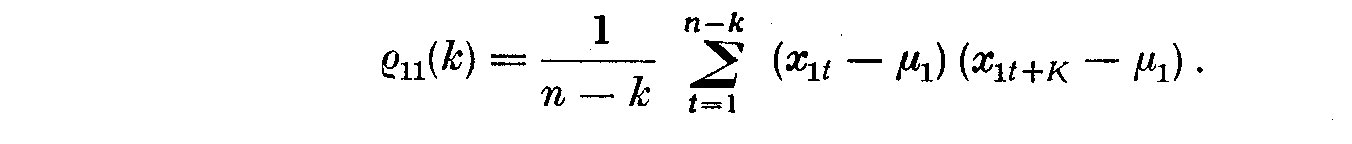
the mean value of X and p(x). We can also write the sample estimate
c_11(k) of the autocovariance of lag K uncorrected for the mean.
(2.3)
where p(x) is the probability density function of the errors and mu_i is
the mean value of X and p(x). We can also write the sample estimate
c_11(k) of the autocovariance of lag K uncorrected for the mean.
 (2.4)
Since c_11(k) is even
(2.4)
Since c_11(k) is even
 (2.5)
If the number of observations n increases indefinitely, c_11(k) becomes the
ensemble autocovariance gamma_11(k). Priestley (1965) points out that C_11(k)
has a bias b(omega) the order m/n, but since most estimates of the spectral
density use only the first m(<<n) values of gamma_11(k), so the bias in
gamma_11(k) is unimportant. If we wish to compute only the autocorrelation,
then we use an unbiased estimate of c_11(k). However, to calculate the power
spectrum of X_1(t) requires a biased estimate of c_11(k) (see designation 3.14
and the immediate discussion), thus a weighted autocorrelation becomes:
(2.5)
If the number of observations n increases indefinitely, c_11(k) becomes the
ensemble autocovariance gamma_11(k). Priestley (1965) points out that C_11(k)
has a bias b(omega) the order m/n, but since most estimates of the spectral
density use only the first m(<<n) values of gamma_11(k), so the bias in
gamma_11(k) is unimportant. If we wish to compute only the autocorrelation,
then we use an unbiased estimate of c_11(k). However, to calculate the power
spectrum of X_1(t) requires a biased estimate of c_11(k) (see designation 3.14
and the immediate discussion), thus a weighted autocorrelation becomes:
 (2.6)
The autocorrelation coefficients rho_11(k) are phi_11(k)=gamma_11(k)/gamma_11(0);
here the same as the regression coefficients of X_1(t) on X_1(t-k). The
cross correlation coefficients rho_12(k) become
(2.6)
The autocorrelation coefficients rho_11(k) are phi_11(k)=gamma_11(k)/gamma_11(0);
here the same as the regression coefficients of X_1(t) on X_1(t-k). The
cross correlation coefficients rho_12(k) become
 (2.7)
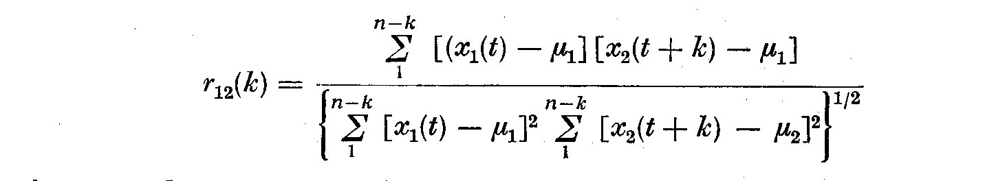
Thus if the time series is stationary and normal, its statistical process, i.e.
the joint distribution of X_1(t) for time t_1, t_2, ..., t_n is characterized
sufficiently by mu_i, sigma_2 and rho_12(k) (Jenkins, 1961). More formally the
estimators gamma_12(k) for rho_12(k) are the ordinary product-moment
correlations between sequences
(2.7)
Thus if the time series is stationary and normal, its statistical process, i.e.
the joint distribution of X_1(t) for time t_1, t_2, ..., t_n is characterized
sufficiently by mu_i, sigma_2 and rho_12(k) (Jenkins, 1961). More formally the
estimators gamma_12(k) for rho_12(k) are the ordinary product-moment
correlations between sequences
 (2.8)
where mu_1 and mu_2 are means calculated from the first n-k and last n-k terms,
respectively. The plots of r_12(k) versus the lag k are called the autocorrelation
functions A_11(k) and r_12(k) against k the cross-correlation functions. It is
worth noting that the means mu_1 and mu_2 must be subtracted to produce
proper autocorrelation coefficients. If we do not remove the sample mean before
calculating the autocovariances it will dominate the contribution to its
cosine transform not only at zero frequency, but also at frequencies close to
zero. A Fourier transform of rho_11(k) will dominate only the zero frequency,
but if there is linear trend present in addition, there will be an additional
contribution to the power at all frequencies, but predominantly at low
frequencies. We note also that if the lag k becomes too large, R_12(k) becomes
erratic in appearance since fewer observations fall into each group, so that
the variance of the estimate increases. Thus resolution cum number of lags
k works in the opposite directions to the variance, and a compromise between
the two must be effected to accurately estimate autocorrelation coefficients.
III. HARMONIC ANALYSIS OF STRICTLY PERIODIC TIME SERIES
The sample autocorrelation function is a difficult quantity to interpret
physically since neighbouring correlations tend to be correlated. We shall try
to look at the time series transformed into the frequency domain. We shall first
decompose a time series that is valid only for strictly periodic phenomena.
After we show how certain types of noisy spectra can be represented, i.e.
we shall estimate a power spectrum of a time series containing both periodic
signals and noise.
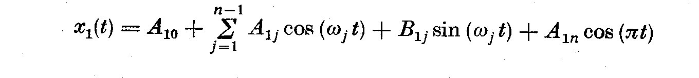
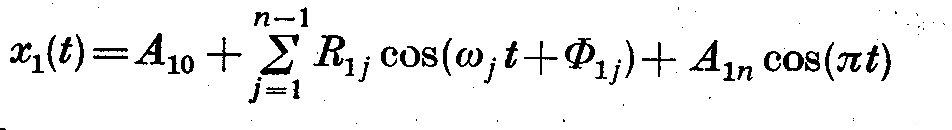
Following Jenkins (1965), we shall unite N = 2n sampling intervals of a
strictly periodic time series (light curve) which will be fitted to a
harmonic regression of the form
(2.8)
where mu_1 and mu_2 are means calculated from the first n-k and last n-k terms,
respectively. The plots of r_12(k) versus the lag k are called the autocorrelation
functions A_11(k) and r_12(k) against k the cross-correlation functions. It is
worth noting that the means mu_1 and mu_2 must be subtracted to produce
proper autocorrelation coefficients. If we do not remove the sample mean before
calculating the autocovariances it will dominate the contribution to its
cosine transform not only at zero frequency, but also at frequencies close to
zero. A Fourier transform of rho_11(k) will dominate only the zero frequency,
but if there is linear trend present in addition, there will be an additional
contribution to the power at all frequencies, but predominantly at low
frequencies. We note also that if the lag k becomes too large, R_12(k) becomes
erratic in appearance since fewer observations fall into each group, so that
the variance of the estimate increases. Thus resolution cum number of lags
k works in the opposite directions to the variance, and a compromise between
the two must be effected to accurately estimate autocorrelation coefficients.
III. HARMONIC ANALYSIS OF STRICTLY PERIODIC TIME SERIES
The sample autocorrelation function is a difficult quantity to interpret
physically since neighbouring correlations tend to be correlated. We shall try
to look at the time series transformed into the frequency domain. We shall first
decompose a time series that is valid only for strictly periodic phenomena.
After we show how certain types of noisy spectra can be represented, i.e.
we shall estimate a power spectrum of a time series containing both periodic
signals and noise.
Following Jenkins (1965), we shall unite N = 2n sampling intervals of a
strictly periodic time series (light curve) which will be fitted to a
harmonic regression of the form
 (3.1)
or
(3.1)
or
 (3.2)
where
(3.2)
where
 The observations are represented by a mixture of sine and cosine waves
whose frequencies are multiples of the fundamental frequency 2 pi / N . Then
The observations are represented by a mixture of sine and cosine waves
whose frequencies are multiples of the fundamental frequency 2 pi / N . Then
 (3.3)
(3.3)
 (3.4)
and
(3.4)
and
 (3.5)
If only a few of the harmonics are used, and the remainder are regarded
as error, then (3.4) and (3.5) give the usual least square estimates of the
constants. The total sum of the squares (variances) about the mean can be
decomposed.
(3.5)
If only a few of the harmonics are used, and the remainder are regarded
as error, then (3.4) and (3.5) give the usual least square estimates of the
constants. The total sum of the squares (variances) about the mean can be
decomposed.
 (3.6)
If we assume no harmonic terms are present, then N/2*R_ij^2 is distributed as
chi-square with two degrees of freedom.
If we define the sample estimate of the autocovariance of lag k uncorrected
for the mean c_11(k) then the sample spectral density function is
(3.6)
If we assume no harmonic terms are present, then N/2*R_ij^2 is distributed as
chi-square with two degrees of freedom.
If we define the sample estimate of the autocovariance of lag k uncorrected
for the mean c_11(k) then the sample spectral density function is
 (3.7)
We can now carry out a harmonic analysis for strictly periodic phenomena as
(3.7)
We can now carry out a harmonic analysis for strictly periodic phenomena as
 (3.8)
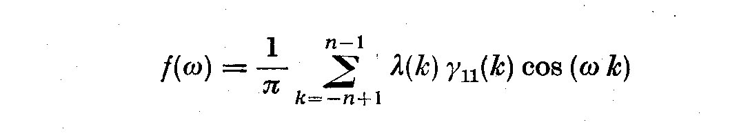
If the series X_1(t) is stationary, and if the number of observations N
increases indefinitely the histogram R_ij becomes a continuous curve
known as the spectral density function f(omega) and, C_11(k) is replaced
by gamma_11(k) so that
(3.8)
If the series X_1(t) is stationary, and if the number of observations N
increases indefinitely the histogram R_ij becomes a continuous curve
known as the spectral density function f(omega) and, C_11(k) is replaced
by gamma_11(k) so that
 (3.9)
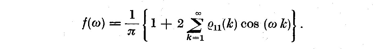
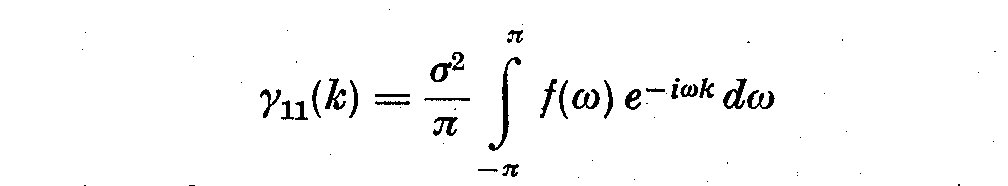
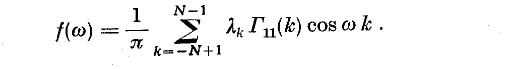
It is worth noting that f(omega) and gamma_11(k) are Fourier transforms of
each other. We have
(3.9)
It is worth noting that f(omega) and gamma_11(k) are Fourier transforms of
each other. We have
 (3.10)
and we write rho_11(k) = gamma(k)/sigma^2
(3.10)
and we write rho_11(k) = gamma(k)/sigma^2
 (3.11)
The Weiner-Khintchine theorem states this more formally: that a function
f (omega) being the integrated spectrum of X (t) has the physical
interpretation that follows from the Fourier expansion of X_1(t)_1 i.e.
(3.11)
The Weiner-Khintchine theorem states this more formally: that a function
f (omega) being the integrated spectrum of X (t) has the physical
interpretation that follows from the Fourier expansion of X_1(t)_1 i.e.
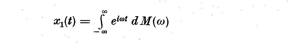 (3.12)
where dM(omega) is an orthogonal stochastic process in the interval
(-infinity, infinity)
with the estimate
(3.12)
where dM(omega) is an orthogonal stochastic process in the interval
(-infinity, infinity)
with the estimate
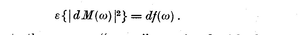 (3.13)
Thus df(omega) represents the average "power" associated with the
components of X_1(t) whose frequencies lie between omega and omega + d omega.
We shall now see why this easy progression in the proof does not
yield valid results for physically meaningful spectra, since simply, the
tenants of the basic assumption of strictly periodic X_1(t) are violated
for stars with irregularly varying light curves.
As we have stated harmonic analysis works only for strictly periodic
phenomena. For mixed time series harmonic analysis does not give a natural
estimate of the spectra. In fact engineers and statisticians know harmonic
analysis of noise or random numbers produces a highly spiked spectrum. For
large sample sizes the mean periodogram I_11(omega) does tend to the spectral
density, but the variance of the fluctuations of I_11(omega) about f(omega)
does not tend to zero as n -> infinity. For a large n, the distribution of
I_11(omega) is a multiple of a chi-squared distribution with two degrees of
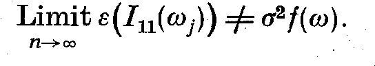
freedom, independently of n. Another way to see that for mixed spectra harmonic
estimates of the periodogram I_11(omega) are spurious is that
(3.13)
Thus df(omega) represents the average "power" associated with the
components of X_1(t) whose frequencies lie between omega and omega + d omega.
We shall now see why this easy progression in the proof does not
yield valid results for physically meaningful spectra, since simply, the
tenants of the basic assumption of strictly periodic X_1(t) are violated
for stars with irregularly varying light curves.
As we have stated harmonic analysis works only for strictly periodic
phenomena. For mixed time series harmonic analysis does not give a natural
estimate of the spectra. In fact engineers and statisticians know harmonic
analysis of noise or random numbers produces a highly spiked spectrum. For
large sample sizes the mean periodogram I_11(omega) does tend to the spectral
density, but the variance of the fluctuations of I_11(omega) about f(omega)
does not tend to zero as n -> infinity. For a large n, the distribution of
I_11(omega) is a multiple of a chi-squared distribution with two degrees of
freedom, independently of n. Another way to see that for mixed spectra harmonic
estimates of the periodogram I_11(omega) are spurious is that
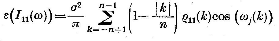 (3.14)
where
(3.14)
where
 As we see, the weights tend to zero as k tends to N, giving erratic and
incorrect estimates. We shall now see a true method of estimating time
series as developed by Weiner (1967), Blackman and Tukey (1958), and others.
IV. ESTIMATION OF MIXED AUTOSPECTRA
We here define a mixed spectra by decomposing F(omega), integrated spectrum
of X_1(t) as
As we see, the weights tend to zero as k tends to N, giving erratic and
incorrect estimates. We shall now see a true method of estimating time
series as developed by Weiner (1967), Blackman and Tukey (1958), and others.
IV. ESTIMATION OF MIXED AUTOSPECTRA
We here define a mixed spectra by decomposing F(omega), integrated spectrum
of X_1(t) as
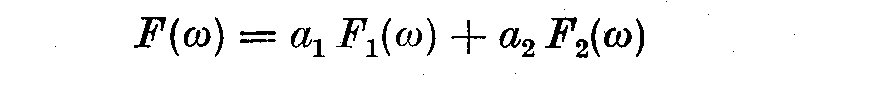 (4.1)
where F_1(omega) is an absolutely continuous function having a derivative
f(omega) also called the spectral density function, and F_2(omega) is a step
function at certain frequencies omega_n, n = 1, 2,... If a = 1, a_2 = 0 the
spectrum is purely continuous; if a_1 = 0, a_2 = 1, it is purely discrete.
If a_1 unequal 0, and a_2 unequal 0 are not constant, then the time
series is said to possess a mixed spectrum. If a process contains
periodic terms and residual processes which in themselves have continuous
spectra, then we have to estimate (1) the number of sine waves, (2)
their amplitudes and frequencies, and (3) the spectral density function
of the residual process.
To estimate mixed spectra one defines both a series lambda(k) as a time
domain window and a spectral window tau(omega) as a window in the frequency
domain. We choose for mixed spectra to define spectral estimates in the form
(4.1)
where F_1(omega) is an absolutely continuous function having a derivative
f(omega) also called the spectral density function, and F_2(omega) is a step
function at certain frequencies omega_n, n = 1, 2,... If a = 1, a_2 = 0 the
spectrum is purely continuous; if a_1 = 0, a_2 = 1, it is purely discrete.
If a_1 unequal 0, and a_2 unequal 0 are not constant, then the time
series is said to possess a mixed spectrum. If a process contains
periodic terms and residual processes which in themselves have continuous
spectra, then we have to estimate (1) the number of sine waves, (2)
their amplitudes and frequencies, and (3) the spectral density function
of the residual process.
To estimate mixed spectra one defines both a series lambda(k) as a time
domain window and a spectral window tau(omega) as a window in the frequency
domain. We choose for mixed spectra to define spectral estimates in the form
 (4.2)
where we assume that the width of the spectral window associated with lambda(k)
is so small that the spectrum is small over the window. We can also write for
gamma_11(k)
(4.2)
where we assume that the width of the spectral window associated with lambda(k)
is so small that the spectrum is small over the window. We can also write for
gamma_11(k)
 (4.3)
Another expression of (4.2) is
(4.3)
Another expression of (4.2) is
 (4.4)
where
(4.4)
where
 (4.5)
with
(4.5)
with
 (4.6)
and
(4.6)
and
 (4.7)
The tau(omega-y) is the spectral window. In changing omega we move the slit
along through the entire frequency range, with a bandwidth +-2 pi/N
about y = omega. Jenkins (1961) gives several physical definitions of
bandwidth which approximate a rectangular band pass window. In general
we will replace the autocovariances gamma_11(k) with the autocorrelations
rho_11(k) so that
(4.7)
The tau(omega-y) is the spectral window. In changing omega we move the slit
along through the entire frequency range, with a bandwidth +-2 pi/N
about y = omega. Jenkins (1961) gives several physical definitions of
bandwidth which approximate a rectangular band pass window. In general
we will replace the autocovariances gamma_11(k) with the autocorrelations
rho_11(k) so that
 (4.8)
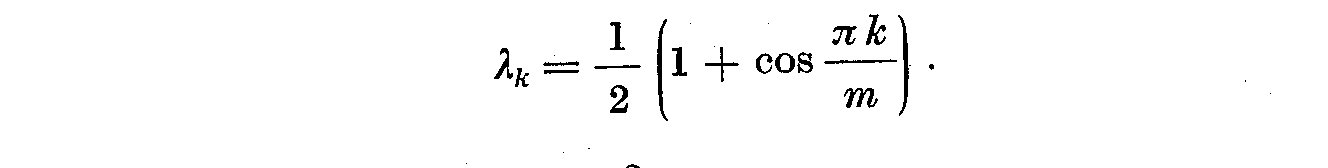
For the choice of moving weights lambda_k, we can choose from a number
of cosine-like series, all nearly the same. We have used
(4.8)
For the choice of moving weights lambda_k, we can choose from a number
of cosine-like series, all nearly the same. We have used
 (4.9)
This weight gives variance f(omega)~ 3m/4n, thus making m small
increases the bandwidth, hence decreasing the variance for this choice
of lambda_12.
This operation can be regarded as a filtering process using a
rectangular-like bandpass with small side lobes in order to increase the
accuracy of the spectral density f(omega). Unless one is faced with
peaky or a steeply slanted spectrum, the exact shape of the window is
not too critical.
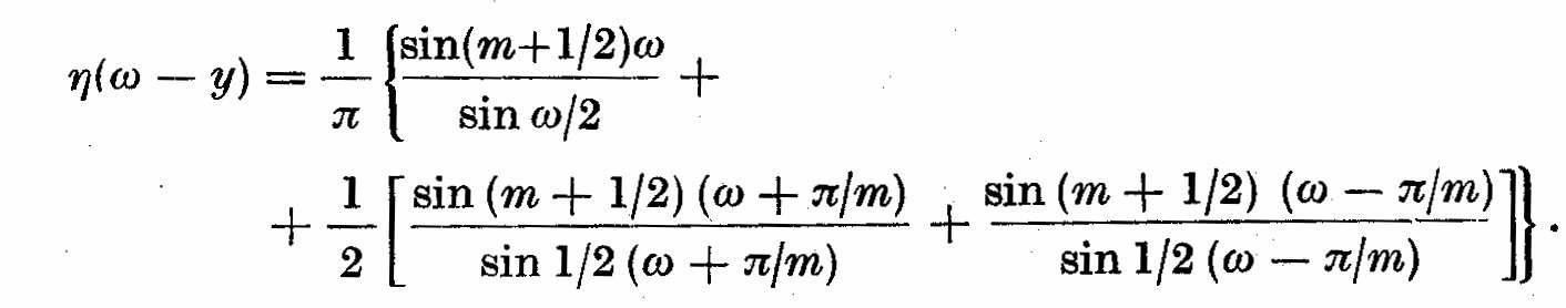
This window (4.9) and others like it tend to a normal distribution,
hence its transform is the same as itself. It retains its shape in both
time and frequency domains. For his particular window, the eta(omega-y)
in (4.1) is given by Jenkins (1961) as
(4.9)
This weight gives variance f(omega)~ 3m/4n, thus making m small
increases the bandwidth, hence decreasing the variance for this choice
of lambda_12.
This operation can be regarded as a filtering process using a
rectangular-like bandpass with small side lobes in order to increase the
accuracy of the spectral density f(omega). Unless one is faced with
peaky or a steeply slanted spectrum, the exact shape of the window is
not too critical.
This window (4.9) and others like it tend to a normal distribution,
hence its transform is the same as itself. It retains its shape in both
time and frequency domains. For his particular window, the eta(omega-y)
in (4.1) is given by Jenkins (1961) as
 (4.10)
Most windows are similar to those generated from the window lambda_12 = 1,
giving a shape similar to the probability density function of a
rectangular random variable. This particular window (4.9) has both small
bandwidths and small side lobes, cutting the leakage of spectral power
from frequencies distant from y = omega, which would distort the true
picture at y = omega_0. It must be emphasized that there are a number of
spectral windows, each with different bandwidths. We shall see later
that filters similar to lambda_12 are used to suppress certain undesirable
features in the spectrum such as power leakage. More important than the
choice of window shape is the choice of the total number of lag k steps,
which we call m. The nature of the analysis attempted here is to use a
fixed run of observations and a fixed sampling interval Delta t. Priestley
(1962) has attempted to establish quantitative expressions for designing
an optimum spectral estimate, involving the relation of variance sigma^2 and
bias b(omega). As we have mentioned earlier, one must first fix the form of
the weight sequence and the number of lags m. A not always realizable
suggestion by Priestley (1962) is to have the bandwidth Bomega not greater
than the width of the narrowest peak of f(omega), more specifically Bomega
is the distance between the `half-power' points in the main lobe.
Blackman and Tukey {1958) discuss an optimal design in terms of sampling
errors of f(omega) assuming a chi-squared distribution with nu degrees, of freedom,
including a measure of f(omega) in terms of variance, but not bias b(omega).
We shall discuss these points later when considering the errors inherent in any
estimate of f(omega). These considerations of sigma^2 and b(omega) are not
strictly applicable to this particular type of power spectrum of light
curves analysis of light curves of irregular variable stars taken from
the astronomy literature. Unless one studies only short period
fluctuations of variable stars, or has several observatories in the
world keeping constant watch on certain stars, one's sampling rate will
always be disturbed by the day-night variation. The weather will also
confound the most diligent observer, and tend to frustrate any decrease
of Delta t even for very long records of light curves.
Jenkins (1965) suggests an empirical method which has been followed in
this work, and which will be illustrated by a few examples and diagrams.
Those who try to determine an optimal m always find that the answers
depend on the spectral density f(omega). We therefore choose an m small
(or large bandwidth). We then increase m and decrease the bandwidth
improving the resolution, stopping when we are satisfied about the
detail of the spectrum (following the suggestion of Priestley). The
matter may be judged in the light of the consideration that the variance
tends to increase with m; we must in fact balance three considerations:
accuracy of spectral estimate (the variance) against the number of lags
m, i.e. the resolution of fine structure in the spectrum. The ideal
method to increase resolution at low frequencies which would amount to
an increase in the total length of data, hence a range of possible
periods of up to 1,000 days. Along with this increase in n we could
safely increase m and still retain a high level of confidence in our
statistical estimates of the spectra. The diurnal variation of the
Earth, infrequent bad weather and the new Moon puts a very real
limitation on an accurate f(omega), without an enormous increase in time
and effort of the observational astronomers.
The irregular nature of the observations that make up a light curve is
dealt with by a subroutine of BOMM that interpolates the time series,
using second differences, at regular intervals Delta t over the range of
observations that one chooses. In pilot studies, we usually choose
several values of Delta t.
We are led finally to conclude this section with the specific
formulation of the spectral density as computed by a BOMM subroutine.
The actual cosine transformation of the autocorrelation is written: -
(4.10)
Most windows are similar to those generated from the window lambda_12 = 1,
giving a shape similar to the probability density function of a
rectangular random variable. This particular window (4.9) has both small
bandwidths and small side lobes, cutting the leakage of spectral power
from frequencies distant from y = omega, which would distort the true
picture at y = omega_0. It must be emphasized that there are a number of
spectral windows, each with different bandwidths. We shall see later
that filters similar to lambda_12 are used to suppress certain undesirable
features in the spectrum such as power leakage. More important than the
choice of window shape is the choice of the total number of lag k steps,
which we call m. The nature of the analysis attempted here is to use a
fixed run of observations and a fixed sampling interval Delta t. Priestley
(1962) has attempted to establish quantitative expressions for designing
an optimum spectral estimate, involving the relation of variance sigma^2 and
bias b(omega). As we have mentioned earlier, one must first fix the form of
the weight sequence and the number of lags m. A not always realizable
suggestion by Priestley (1962) is to have the bandwidth Bomega not greater
than the width of the narrowest peak of f(omega), more specifically Bomega
is the distance between the `half-power' points in the main lobe.
Blackman and Tukey {1958) discuss an optimal design in terms of sampling
errors of f(omega) assuming a chi-squared distribution with nu degrees, of freedom,
including a measure of f(omega) in terms of variance, but not bias b(omega).
We shall discuss these points later when considering the errors inherent in any
estimate of f(omega). These considerations of sigma^2 and b(omega) are not
strictly applicable to this particular type of power spectrum of light
curves analysis of light curves of irregular variable stars taken from
the astronomy literature. Unless one studies only short period
fluctuations of variable stars, or has several observatories in the
world keeping constant watch on certain stars, one's sampling rate will
always be disturbed by the day-night variation. The weather will also
confound the most diligent observer, and tend to frustrate any decrease
of Delta t even for very long records of light curves.
Jenkins (1965) suggests an empirical method which has been followed in
this work, and which will be illustrated by a few examples and diagrams.
Those who try to determine an optimal m always find that the answers
depend on the spectral density f(omega). We therefore choose an m small
(or large bandwidth). We then increase m and decrease the bandwidth
improving the resolution, stopping when we are satisfied about the
detail of the spectrum (following the suggestion of Priestley). The
matter may be judged in the light of the consideration that the variance
tends to increase with m; we must in fact balance three considerations:
accuracy of spectral estimate (the variance) against the number of lags
m, i.e. the resolution of fine structure in the spectrum. The ideal
method to increase resolution at low frequencies which would amount to
an increase in the total length of data, hence a range of possible
periods of up to 1,000 days. Along with this increase in n we could
safely increase m and still retain a high level of confidence in our
statistical estimates of the spectra. The diurnal variation of the
Earth, infrequent bad weather and the new Moon puts a very real
limitation on an accurate f(omega), without an enormous increase in time
and effort of the observational astronomers.
The irregular nature of the observations that make up a light curve is
dealt with by a subroutine of BOMM that interpolates the time series,
using second differences, at regular intervals Delta t over the range of
observations that one chooses. In pilot studies, we usually choose
several values of Delta t.
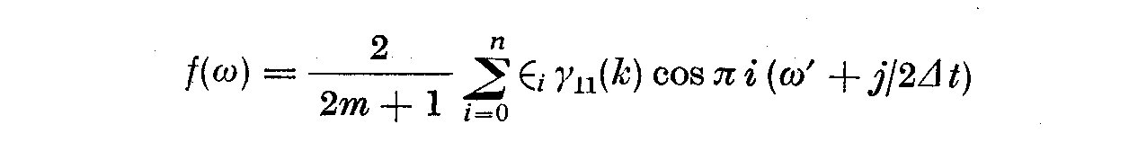
We are led finally to conclude this section with the specific
formulation of the spectral density as computed by a BOMM subroutine.
The actual cosine transformation of the autocorrelation is written: -
 (4.11)
where Epsilon_1 = 1/2 if i = 0, Epsilon_1 = 1 otherwise; j = 0, 1, ... , 1', 1'
is the greatest integer such that omega' + l'/ 2 Delta t <= omega_N
where omega' is the low frequency limit, usually 0 and omega_N is
the Nyquist frequency.
Jenkins (1961) observes that the logarithmic transformation of the spectral
density f(omega) produces a distribution whose variance is nearly independent
of the frequency. We see that
(4.11)
where Epsilon_1 = 1/2 if i = 0, Epsilon_1 = 1 otherwise; j = 0, 1, ... , 1', 1'
is the greatest integer such that omega' + l'/ 2 Delta t <= omega_N
where omega' is the low frequency limit, usually 0 and omega_N is
the Nyquist frequency.
Jenkins (1961) observes that the logarithmic transformation of the spectral
density f(omega) produces a distribution whose variance is nearly independent
of the frequency. We see that
 (4.12)
where beta_i depends on the window used for the spectral estimate and n is
the total number of observations. If we then write an expression independent of
the frequency
(4.12)
where beta_i depends on the window used for the spectral estimate and n is
the total number of observations. If we then write an expression independent of
the frequency
 (4.13)
Log_10 f(omega) produces estimates that do not rely so heavily upon
normality, in fact it produces distributions closer to normality. It is
assumed that the errors here are produced by the variance and not by
leakage of power from other frequencies or by aliasing. It is worth
noting that this leads us easily to the method engineers use for
estimating spectral power since
(4.13)
Log_10 f(omega) produces estimates that do not rely so heavily upon
normality, in fact it produces distributions closer to normality. It is
assumed that the errors here are produced by the variance and not by
leakage of power from other frequencies or by aliasing. It is worth
noting that this leads us easily to the method engineers use for
estimating spectral power since
 (4.14)
We see that an increase of power by a factor of 2 is equivalent of a change
of 3 decibels.
V. ESTIMATION OF MIXED CROSS SPECTRA
Often we need either to compare two empirical time series X_1(t) and
X_2(t) that arise in similar fashions. To do this, we shall show how one
estimates the cross spectrum. We shall show now that if X_1(t) and X_2(t)
do not have similar origins, then one can estimate the gain of a system,
and perhaps the coherent energy. Let one of the time series X_1(t) be a
theoretical complex input and X_2(t) the actual recording of the light
curve. We can write
(4.14)
We see that an increase of power by a factor of 2 is equivalent of a change
of 3 decibels.
V. ESTIMATION OF MIXED CROSS SPECTRA
Often we need either to compare two empirical time series X_1(t) and
X_2(t) that arise in similar fashions. To do this, we shall show how one
estimates the cross spectrum. We shall show now that if X_1(t) and X_2(t)
do not have similar origins, then one can estimate the gain of a system,
and perhaps the coherent energy. Let one of the time series X_1(t) be a
theoretical complex input and X_2(t) the actual recording of the light
curve. We can write
 (5.1)
where n(t) is the noise term which arises because other input variables
are not well controlled. If the fluctuations in X_1(t) are not too large,
then we linearize the above equation to:
(5.1)
where n(t) is the noise term which arises because other input variables
are not well controlled. If the fluctuations in X_1(t) are not too large,
then we linearize the above equation to:
 (5.2)
where n(t) now contains quadratic and higher terms. This relationship is a
linear dynamic equation, the regression or impulse response omega(u) can be
estimated in several ways, by changing X_1(t) by a well defined step pattern
or sinusoidally. In the case of the latter we let X_1(t) = delta cos omega t
and
(5.2)
where n(t) now contains quadratic and higher terms. This relationship is a
linear dynamic equation, the regression or impulse response omega(u) can be
estimated in several ways, by changing X_1(t) by a well defined step pattern
or sinusoidally. In the case of the latter we let X_1(t) = delta cos omega t
and
 (5.3)
then the transfer function becomes
(5.3)
then the transfer function becomes
 (5.4)
T(i omega) is the transfer function, G(omega) the gain and Phi(omega) the phase
shift. If n(t) is small, the gain G(omega) may be obtained from the ratio of
the amplitudes of the output and input, and Phi(omega) by matching up the two
waves. In this case we used a sine wave generator to actuate X_1(t) and sweep
out a range of frequencies to generate all the information.
We shall now estimate omega(u) from the existing noisy fluctuations in X_1(t)
and X_2(t). These two series are now given to be stationary time series, and
X_1(t) and n(t) are uncorrelated, so we can write the crosscovariance by
multiplying (5.2) by X_1(t - k) and averaging
(5.4)
T(i omega) is the transfer function, G(omega) the gain and Phi(omega) the phase
shift. If n(t) is small, the gain G(omega) may be obtained from the ratio of
the amplitudes of the output and input, and Phi(omega) by matching up the two
waves. In this case we used a sine wave generator to actuate X_1(t) and sweep
out a range of frequencies to generate all the information.
We shall now estimate omega(u) from the existing noisy fluctuations in X_1(t)
and X_2(t). These two series are now given to be stationary time series, and
X_1(t) and n(t) are uncorrelated, so we can write the crosscovariance by
multiplying (5.2) by X_1(t - k) and averaging
 (5.5)
where gamma_12(k) is the crosscovariance function of lag k between X_1(t) and
X_2(t), and gamma_11(k-u) is the autocovariance function. If gamma_12(k) and
gamma_11(k-u) are known, then omega(u) may be estimated by solving (5.5),
usually called the Weiner-Hopf equation. If we calculate the Fourier transform
of both sides, T(omega) is then
(5.5)
where gamma_12(k) is the crosscovariance function of lag k between X_1(t) and
X_2(t), and gamma_11(k-u) is the autocovariance function. If gamma_12(k) and
gamma_11(k-u) are known, then omega(u) may be estimated by solving (5.5),
usually called the Weiner-Hopf equation. If we calculate the Fourier transform
of both sides, T(omega) is then
 (5.6)
where f_12(omega) is the cross spectral density function, and sigma_1 and
sigma_2 are the standard deviations of X_1(t) and X_2(t). The spectral density
f_12(omega) is given by
(5.6)
where f_12(omega) is the cross spectral density function, and sigma_1 and
sigma_2 are the standard deviations of X_1(t) and X_2(t). The spectral density
f_12(omega) is given by
 (5.7)
We have shown that the frequency response tau(omega) is given by the ratio of
the cross spectral density and the input auto spectrum. We now write gamma_12(k) as:
(5.7)
We have shown that the frequency response tau(omega) is given by the ratio of
the cross spectral density and the input auto spectrum. We now write gamma_12(k) as:
 (5.8)
We have already defined gamma_11(k) and f_11(omega) in an earlier section of
the paper. Since gamma_12(k) unequal gamma_21(k) in general, then (5.7) gives
both a cosine and sine transform of the crosscorrelation
(5.8)
We have already defined gamma_11(k) and f_11(omega) in an earlier section of
the paper. Since gamma_12(k) unequal gamma_21(k) in general, then (5.7) gives
both a cosine and sine transform of the crosscorrelation
 (5.9)
(5.9)
 (5.10)
where
(5.10)
where
 (5.11)
 (5.12)
and
(5.12)
and
 (5.13)
In this case W_12(omega) is the quadrature or out-of-phase spectrum, and Z_12(omega)
is called the co- or in-phase spectrum. Using (5.6) and (5.8) we can write the
gain G(omega) and phase Phi(omega) as
(5.13)
In this case W_12(omega) is the quadrature or out-of-phase spectrum, and Z_12(omega)
is called the co- or in-phase spectrum. Using (5.6) and (5.8) we can write the
gain G(omega) and phase Phi(omega) as
 (5.14)
 (5.15)
Tan Phi_i(omega) here is the phase difference. This formulation is due to Munk,
et al. (1959). If we are examining the covariance between two stationary time
series X_1(t) and X_2(t) and not as input and output of some linear system,
one usually plots the coherence R^2(omega), which is normalized to run between
0 and 1 so that
(5.15)
Tan Phi_i(omega) here is the phase difference. This formulation is due to Munk,
et al. (1959). If we are examining the covariance between two stationary time
series X_1(t) and X_2(t) and not as input and output of some linear system,
one usually plots the coherence R^2(omega), which is normalized to run between
0 and 1 so that
 (5.16)
The coherency R^2(omega) is analogous to the correlation coefficient calculated
at each frequency omega. The spectrum of the noise term n(t) in (5.2) is now
(5.16)
The coherency R^2(omega) is analogous to the correlation coefficient calculated
at each frequency omega. The spectrum of the noise term n(t) in (5.2) is now
 (5.17)
which is analogous to the residual sum of squares in linear regression.
(5.17)
which is analogous to the residual sum of squares in linear regression.
 (5.18)
We see if R^2(omega) is large, the noise spectral density is small relative
to the output spectral density and vice versa. We can also write R^2(omega) as
(5.18)
We see if R^2(omega) is large, the noise spectral density is small relative
to the output spectral density and vice versa. We can also write R^2(omega) as
 (5.19)
If G(omega) is specified, the coherency is large if the signal-to-noise ratio
is large, that is S(omega)/N(omega)
(5.19)
If G(omega) is specified, the coherency is large if the signal-to-noise ratio
is large, that is S(omega)/N(omega)
 (5.20)
Munk, Snodgrass and Tucker (1959) point out that, if both X_1(t) and
X_2(t) are identical and simultaneous, Z_12(omega) = +1, W_12(omega) = 0.
If they are identical but there is a time lag in one record corresponding to a
phase difference Phi(omega), then the coherence is +1.
Jenkins (1965) points out that positive cross correlations will result in a
high frequency cross amplitude spectrum with most of its power at low
frequencies; negative cross correlations will results in a high-frequency
cross amplitude spectrum.
We follow Jenkins (1963, 1965) to choose w(n) in (5.2) so that the
integrated squared error is minimized, and that (5.21) is small compared
to some Epsilon
(5.20)
Munk, Snodgrass and Tucker (1959) point out that, if both X_1(t) and
X_2(t) are identical and simultaneous, Z_12(omega) = +1, W_12(omega) = 0.
If they are identical but there is a time lag in one record corresponding to a
phase difference Phi(omega), then the coherence is +1.
Jenkins (1965) points out that positive cross correlations will result in a
high frequency cross amplitude spectrum with most of its power at low
frequencies; negative cross correlations will results in a high-frequency
cross amplitude spectrum.
We follow Jenkins (1963, 1965) to choose w(n) in (5.2) so that the
integrated squared error is minimized, and that (5.21) is small compared
to some Epsilon
 (5.21)
and
(5.21)
and
 (5.22)
Here the ensemble cross covariances gamma_12(k) are replaced by the sample
cross covariances Z_12(k). Since X_1(t) and X_2(t) are not phase shifted sine
waves, but stationary time series, we must introduce a weight function
lambda(k) as in the univariate spectral analysis. We then write the
estimates for the co-spectra, quadrature and auto-spectra as
(5.22)
Here the ensemble cross covariances gamma_12(k) are replaced by the sample
cross covariances Z_12(k). Since X_1(t) and X_2(t) are not phase shifted sine
waves, but stationary time series, we must introduce a weight function
lambda(k) as in the univariate spectral analysis. We then write the
estimates for the co-spectra, quadrature and auto-spectra as
 (5.23)
 (5.24)
 (5.25)
where alpha_12(k) and beta_12(k) are estimates of alpha_12 and beta_12
as defined earlier in (5.12) and (5.13).
It has been pointed out by Jenkins (1965) that coherencies may sometimes
be low because of the influences of the individual autospectra. One can take
two independent time series and produce large coherence between them arising
from peaks in the individual spectra or if the bandwidth is too small. However,
we can calculate the autospectra first, then pre-filter each series to make
their spectra move nearly uniform or white. This leads to a large increase in
accuracy in the estimation of coherency. If one likes to think of an input
function into the atmosphere oŁ a star as some type of periodic wave, then
following Munk and Cartwright (1966) we can separate the estimate of the energy
into two parts, namely
(5.25)
where alpha_12(k) and beta_12(k) are estimates of alpha_12 and beta_12
as defined earlier in (5.12) and (5.13).
It has been pointed out by Jenkins (1965) that coherencies may sometimes
be low because of the influences of the individual autospectra. One can take
two independent time series and produce large coherence between them arising
from peaks in the individual spectra or if the bandwidth is too small. However,
we can calculate the autospectra first, then pre-filter each series to make
their spectra move nearly uniform or white. This leads to a large increase in
accuracy in the estimation of coherency. If one likes to think of an input
function into the atmosphere oŁ a star as some type of periodic wave, then
following Munk and Cartwright (1966) we can separate the estimate of the energy
into two parts, namely
 (5.26)
and
(5.26)
and
 (5.27)
The latter will be effectively noise energy, but may contain energy coherent
with other input functions.
VI. FILTERS
Once the basic spectrum has been created and stabilized for a fixed m
and Delta t it becomes important to examine further the processes that tend
to distort the true nature of f(omega). We shall then show it is possible
to construct a digital filter U_k so that convolution upon the data in
the time domain will eliminate unwanted spectral energy at some
specified frequency. If we generate a series which we shall term our
filter, and given our light curve X_1(t), we then create a new series
W_j(t) by the process described. We can write W_j(t) as
(5.27)
The latter will be effectively noise energy, but may contain energy coherent
with other input functions.
VI. FILTERS
Once the basic spectrum has been created and stabilized for a fixed m
and Delta t it becomes important to examine further the processes that tend
to distort the true nature of f(omega). We shall then show it is possible
to construct a digital filter U_k so that convolution upon the data in
the time domain will eliminate unwanted spectral energy at some
specified frequency. If we generate a series which we shall term our
filter, and given our light curve X_1(t), we then create a new series
W_j(t) by the process described. We can write W_j(t) as
 (6.1)
where
(6.1)
where
 p' being the number of terms by which the weight factors are advanced
for unit increase in 1/(l' + 1) is a normalization factor. If we want
weights that are symmetrical, then W_j assumes the following form
p' being the number of terms by which the weight factors are advanced
for unit increase in 1/(l' + 1) is a normalization factor. If we want
weights that are symmetrical, then W_j assumes the following form
 (6.2)
where
(6.2)
where
 We can construct also a frequency response function T(omega) to accept or
reject any range of frequencies so that
We can construct also a frequency response function T(omega) to accept or
reject any range of frequencies so that
 (6.3)
The BOMM programme generates these series of moving weights either for
use as lag windows or as filters. We have the choice of symmetrical
filters or those fading to the left or right. If we want a high-pass or
low-pass filter, then for some frequency f, the terms are multiplied by a
factor which gives a filter whose transmission is 6 db (1/2 amplitude).
Thus: --
(6.3)
The BOMM programme generates these series of moving weights either for
use as lag windows or as filters. We have the choice of symmetrical
filters or those fading to the left or right. If we want a high-pass or
low-pass filter, then for some frequency f, the terms are multiplied by a
factor which gives a filter whose transmission is 6 db (1/2 amplitude).
Thus: --
 (6.4)
(6.4)
 (6.5)
If we want a low pass filter to be convolved in equation (6.1), then we write
(6.5)
If we want a low pass filter to be convolved in equation (6.1), then we write
 (6.6)
and for a high pass filter
(6.6)
and for a high pass filter
 (6.7)
where Epsilon_j = 1/2 for j = 0 and Epsilon_j = 1 otherwise;
delta(j) = 1 for j = 0 and 0 otherwise.
As we stated earlier, the filter type is determined by the sharpness of
cut-off and by the side band characteristics. The amplitude response of
any filter can be obtained taking its cosine transform. It may be worthwhile
explaining some of the conditions which necessitate the use of filters, such
as the removal of trends, leakage of power from high frequencies due to aliasing.
Often non-stationarity of time series may be due to the presence of a linear
trend. In general, one can use a high-pass digital filter to suppress low
frequency trends and then go on to perform a spectral analysis of the residual
series. Another use of filters in time series analysis is where one suspects
that a series consists of a mixture of stationary series, i.e. differing
frequency bands may have different physical origins. In such a case, we can
construct a series of digital band pass filters to separate the original
spectrum into several distinct spectra.
A more complete discussion of the use of filters of all types will come
in the next section with a discussion of the errors involved in calculating
the spectral density.
VII. ERRORS IN SPECTRAL DENSITY ESTIMATES
Munk, Snodgrass and Tucker (1959) have given several quantitative
estimates of errors in spectral density. We shall deal with those errors
that are due to random errors, the properties of the spectral window
lambda(k), leakage of power due to aliasing, and give some treatment of
systematic errors. Within the range of this examination is the problem
of detecting signals in the presence of noise, i.e. estimation of the
range of error allowable for any peak that appears in the mixed spectra.
Parzen (1961) gives some design relations in terms of the signal to
noise estimate, i.e.
(6.7)
where Epsilon_j = 1/2 for j = 0 and Epsilon_j = 1 otherwise;
delta(j) = 1 for j = 0 and 0 otherwise.
As we stated earlier, the filter type is determined by the sharpness of
cut-off and by the side band characteristics. The amplitude response of
any filter can be obtained taking its cosine transform. It may be worthwhile
explaining some of the conditions which necessitate the use of filters, such
as the removal of trends, leakage of power from high frequencies due to aliasing.
Often non-stationarity of time series may be due to the presence of a linear
trend. In general, one can use a high-pass digital filter to suppress low
frequency trends and then go on to perform a spectral analysis of the residual
series. Another use of filters in time series analysis is where one suspects
that a series consists of a mixture of stationary series, i.e. differing
frequency bands may have different physical origins. In such a case, we can
construct a series of digital band pass filters to separate the original
spectrum into several distinct spectra.
A more complete discussion of the use of filters of all types will come
in the next section with a discussion of the errors involved in calculating
the spectral density.
VII. ERRORS IN SPECTRAL DENSITY ESTIMATES
Munk, Snodgrass and Tucker (1959) have given several quantitative
estimates of errors in spectral density. We shall deal with those errors
that are due to random errors, the properties of the spectral window
lambda(k), leakage of power due to aliasing, and give some treatment of
systematic errors. Within the range of this examination is the problem
of detecting signals in the presence of noise, i.e. estimation of the
range of error allowable for any peak that appears in the mixed spectra.
Parzen (1961) gives some design relations in terms of the signal to
noise estimate, i.e.
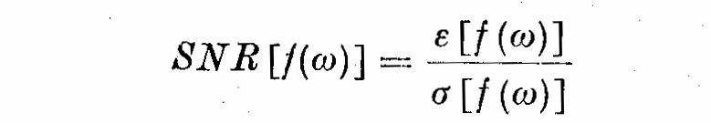 (7.1)
We see the SNR[f(omega)] is the mean divided by the standard deviation (or the
reciprocal) of the coefficient of variation of the random variable f(omega). If
f(omega) is normally distributed and we seek to obtain a 95% confidence level
for our spectral estimates, then we can estimate SNR[f(omega)] in terms of
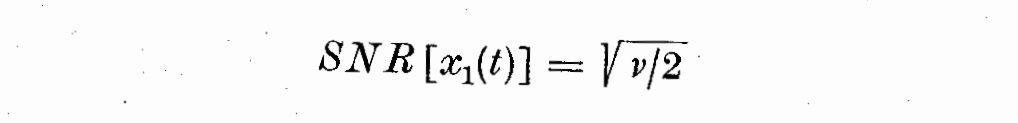
equivalent degrees of freedom. If X_1(t) is a random variable (i.e. Gaussian noise)
which has a chi-squared distribution with nu degrees of freedom, then
(7.1)
We see the SNR[f(omega)] is the mean divided by the standard deviation (or the
reciprocal) of the coefficient of variation of the random variable f(omega). If
f(omega) is normally distributed and we seek to obtain a 95% confidence level
for our spectral estimates, then we can estimate SNR[f(omega)] in terms of
equivalent degrees of freedom. If X_1(t) is a random variable (i.e. Gaussian noise)
which has a chi-squared distribution with nu degrees of freedom, then
 (7.2)
and
(7.2)
and
 (7.3)
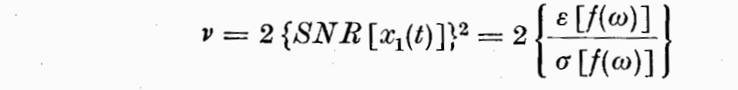
If X_1(t) is a positive random variable, then nu is just the equivalent
degree of freedom.
Several authors put forward their views on design relations to maximize
SNR[f(omega)] under various circumstances (Parzen, 1961; Priestley, 1962;
1965), but we shall have to outline this in more detail later because of
the peculiar nature of the light curves of T Tauri stars and the fixed
amount and nature of the data available. The assumption of a chi-squared
distribution is approximately correct where f(omega) can be expressed as a
weighted sum of chi^2-variables. It seems a similar method of treatment is
to sum the squares of amplitudes of the components of a Fourier series.
(7.3)
If X_1(t) is a positive random variable, then nu is just the equivalent
degree of freedom.
Several authors put forward their views on design relations to maximize
SNR[f(omega)] under various circumstances (Parzen, 1961; Priestley, 1962;
1965), but we shall have to outline this in more detail later because of
the peculiar nature of the light curves of T Tauri stars and the fixed
amount and nature of the data available. The assumption of a chi-squared
distribution is approximately correct where f(omega) can be expressed as a
weighted sum of chi^2-variables. It seems a similar method of treatment is
to sum the squares of amplitudes of the components of a Fourier series.
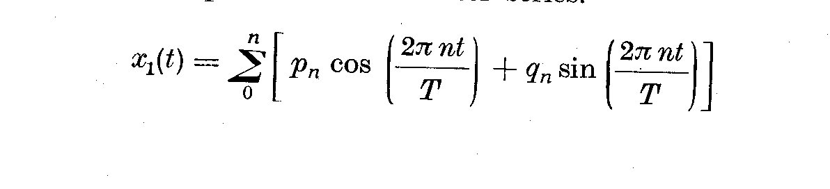 (7.4)
where n = 0, 1, 2 ... , and the energy density varies slowly with the
frequency separation 1/T of the harmonics. Then p_n and q_n, are normal
and p_n^2 = q_n^2 = true energy density/T, i.e.
(7.4)
where n = 0, 1, 2 ... , and the energy density varies slowly with the
frequency separation 1/T of the harmonics. Then p_n and q_n, are normal
and p_n^2 = q_n^2 = true energy density/T, i.e.
 (7.5)
Thus for p harmonics, the number of degrees of freedom nu = 2p, and from
thee chi-squared distribution "confidence limits" can be calculated. This is
because the chi-squared distribution gives
(7.5)
Thus for p harmonics, the number of degrees of freedom nu = 2p, and from
thee chi-squared distribution "confidence limits" can be calculated. This is
because the chi-squared distribution gives
 (7.6)
The effective number of degrees of a record is approximately nu. These
ideas can be used with tables given in Blackman and Tukey (1957) to
calculate the random errors based on the assumptions above. Thus
(7.6)
The effective number of degrees of a record is approximately nu. These
ideas can be used with tables given in Blackman and Tukey (1957) to
calculate the random errors based on the assumptions above. Thus
 (7.7)
It seems likely that one must consider both the bias and variance when
carrying out practical estimates of the spectral density f(omega), but it
is difficult to formulate quantitatively any practical numerical
formulae due to the presence in f(omega) of non-random statistical errors,
i.e. side band leakage for which f(omega) differs with the type of spectral
window chosen, aliasing. The problems of power leakage from peaks at
frequencies > omega_N confuse the estimate at neighbouring frequencies
omega_N +- Delta omega. Parzen (1961) and Priestley (1962) both use a formula
(7.7)
It seems likely that one must consider both the bias and variance when
carrying out practical estimates of the spectral density f(omega), but it
is difficult to formulate quantitatively any practical numerical
formulae due to the presence in f(omega) of non-random statistical errors,
i.e. side band leakage for which f(omega) differs with the type of spectral
window chosen, aliasing. The problems of power leakage from peaks at
frequencies > omega_N confuse the estimate at neighbouring frequencies
omega_N +- Delta omega. Parzen (1961) and Priestley (1962) both use a formula
 (7.8)
to give an estimate at a particular frequency that does not have more
than a 10% proportional error at the 95% confidence level. In this
matter the variance is defined by
(7.8)
to give an estimate at a particular frequency that does not have more
than a 10% proportional error at the 95% confidence level. In this
matter the variance is defined by
 (7.9)
and the bias is given as
(7.9)
and the bias is given as
 (7.10)
where lambda(theta-omega) is the weight function.
Implementation of these formulae for eta(omega) and b(omega) rest critically
on ones choice of the width of the weight function lambda(k). In fact since
both n and b are fixed for the light curves, it is possible to calculate
optimum lags m for a given spectra, if we accept the mean square error
at frequency omega as
(7.10)
where lambda(theta-omega) is the weight function.
Implementation of these formulae for eta(omega) and b(omega) rest critically
on ones choice of the width of the weight function lambda(k). In fact since
both n and b are fixed for the light curves, it is possible to calculate
optimum lags m for a given spectra, if we accept the mean square error
at frequency omega as
 (7.11)
But it cannot be denied that other sources of error creep in as we have
mentioned earlier, and the chi-squared error estimates only account for
one source of error, those of a random nature.
The difficulty is that both eta(omega) and b(omega) are asymptotically
proportional to f(omega). The method we have used is to vary the resolution
until increasing m any further does not reveal any more features in the
spectra, while at the same time attempting to prewhiten the spectra as much as
possible, as suggested by Blackman and Tukey (1957). This is done during Stage
II of the estimation process, which is mostly exploratory.
Pre-whitening is useful in eliminating the systematic errors that occur
due to the curvature of f(omega). If f(omega) is flat, or varies linearly with
frequency, then epsilon [f(omega)] = f(omega). If not, then spectral energy
diffuses down toward lower spectral levels (Munk et al., 1959) and one must
worry about leakage of power from higher frequencies to lower frequencies. We
shall now discuss the question of leakage in the estimates of spectral density.
The window we choose lambda(k) is usually some kind of polynomial which
vanishes at a finite number of points. Its main lobe centering on a band of
frequencies over which we wish to estimate f(omega) is inevitably accompanied
by side bands or minor lobes, which allow leakage from the part of the spectrum
outside the desired band to affect our estimate inside the band. This can be
cured by taking two estimates, one with the side lobes positive, the other
negative.
One of the more critical problems recognised by Tukey is aliasing; or
the problem of sampling at discrete intervals Delta t. It is equivalent to
multiplying the record with spikes with a frequency 1 / Delta t, so that sum
and difference frequencies are produced. An analysis for energy density
at any frequency f will also include the densities near frequencies:
1 / Delta t - f_0, 1 / Delta t + f_0, 2 / Delta t + f_0, ...etc
One of the major uses of filters comes in dealing with leakage of powers
associated with aliasing caused by the loss of information at frequencies
above the Nyquist frequency, namely when omega_N = pi / Delta t,
or f = 1/2 Delta t cycles per day.
(7.11)
But it cannot be denied that other sources of error creep in as we have
mentioned earlier, and the chi-squared error estimates only account for
one source of error, those of a random nature.
The difficulty is that both eta(omega) and b(omega) are asymptotically
proportional to f(omega). The method we have used is to vary the resolution
until increasing m any further does not reveal any more features in the
spectra, while at the same time attempting to prewhiten the spectra as much as
possible, as suggested by Blackman and Tukey (1957). This is done during Stage
II of the estimation process, which is mostly exploratory.
Pre-whitening is useful in eliminating the systematic errors that occur
due to the curvature of f(omega). If f(omega) is flat, or varies linearly with
frequency, then epsilon [f(omega)] = f(omega). If not, then spectral energy
diffuses down toward lower spectral levels (Munk et al., 1959) and one must
worry about leakage of power from higher frequencies to lower frequencies. We
shall now discuss the question of leakage in the estimates of spectral density.
The window we choose lambda(k) is usually some kind of polynomial which
vanishes at a finite number of points. Its main lobe centering on a band of
frequencies over which we wish to estimate f(omega) is inevitably accompanied
by side bands or minor lobes, which allow leakage from the part of the spectrum
outside the desired band to affect our estimate inside the band. This can be
cured by taking two estimates, one with the side lobes positive, the other
negative.
One of the more critical problems recognised by Tukey is aliasing; or
the problem of sampling at discrete intervals Delta t. It is equivalent to
multiplying the record with spikes with a frequency 1 / Delta t, so that sum
and difference frequencies are produced. An analysis for energy density
at any frequency f will also include the densities near frequencies:
1 / Delta t - f_0, 1 / Delta t + f_0, 2 / Delta t + f_0, ...etc
One of the major uses of filters comes in dealing with leakage of powers
associated with aliasing caused by the loss of information at frequencies
above the Nyquist frequency, namely when omega_N = pi / Delta t,
or f = 1/2 Delta t cycles per day.
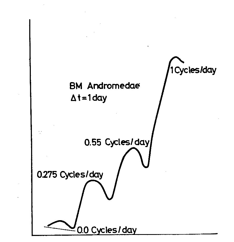
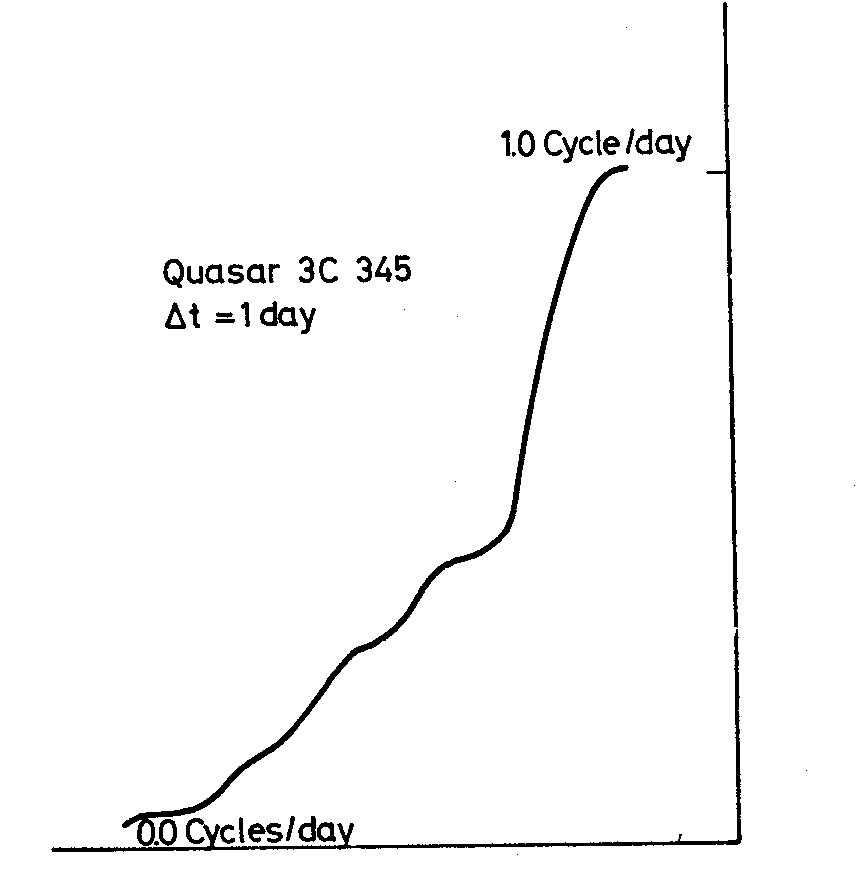 Fig. 1 Fig. 2
Since there is no information available about X_1(t) between the data
points, there is no means of estimating the amplitude of frequencies
higher than the Nyquist frequency. In fact at frequency f_N we are
unable to estimate, since at the Nyquist frequency, f(omega_N) is
confused with all the frequencies that are indistinguishable from
omega_N. If f*(omega) is the spectral density corresponding to X(t),
then the spectral density of the sampled trace is
Fig. 1 Fig. 2
Since there is no information available about X_1(t) between the data
points, there is no means of estimating the amplitude of frequencies
higher than the Nyquist frequency. In fact at frequency f_N we are
unable to estimate, since at the Nyquist frequency, f(omega_N) is
confused with all the frequencies that are indistinguishable from
omega_N. If f*(omega) is the spectral density corresponding to X(t),
then the spectral density of the sampled trace is
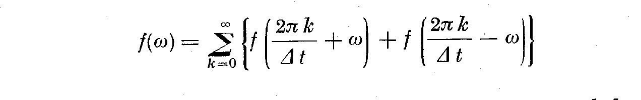 (7.12)
We see the sampled spectrum is obtained by folding the unsampled
spectrum about even multiples (2 pi k)/(Delta t) of f and adding this
contribution in the range (0, omega_N) Thus to be able to measure f*(omega)
in (0, omega_N) we must hope that that f(omega)~~0 for omega > omega_N
In our case it is certain that there is a need to use a low pass
filter to cut any peaks that may occur near f_N. The details of this
process and the practical results of it will be shown when we present
the details of the power spectra for the particular T Tauri stars. The
use of different Delta t's in calculating pilot spectra will tell us if
we are in danger of confusing f(omega) due to higher energies at higher
frequencies.
REFERENCES
Blackman, R. B. and Tukey, J. W., 1958, The Measurement of Power Spectra. Dover
Publications.
Bullard, E. C. et al, 1966, A User's Guide to BOMM. A Series of Programs for
the Analysis of Time Series. Institute of Geophysics and Planetary
Physics, La Jolla.
Herbig, G. H., 1962, Adv. Astr. Astrophys. 1, 47.
Jenkins, G. M., 1961, Technometrics, 3, 167.
Jenkins, G. M., 1963, Technometrics, 5, 227.
Jenkins, G. M., 1965, Applied Statistics, 14, 205.
Munk, W. H., Snodgrass, F. E. and Tucker, M. J., 1959, Bull. Scripps Inst.
Oceanography, 7, 283.
Munk, W. H. and Cartwright, D. E., 1966, Phil. Trans. R. Soc. London, A 259, 533.
Parzen, E., 1961, Technometrics, 3, 167.
Priestley, M. B., 1962, Technometrics, 4, 551.
Priestley, M. B., 1965, Applied Statistics, 14, 33.
Tukey, J. W., 1961, Technometrics, 3, 191.
Weiner, N., 1967, Time Series, Dover Publications.
DISCUSSION
Detre: How is it possible, that the analyses of the same observational material,
by the same method, executed by two different teams - as I mentioned
in my introductory report - lead to opposite results for mu Cephei?
Plagemann: I have not read these contributions, but I shall study them soon.
Herbig: Does your technique recover the periods of a few days found by
Hoffmeister when you analyze the observations of southern RW Aurigae-type
variables made by him ?
Plagemann: I have not yet analyzed his data, although the material is already
on computer cards. It will be done when I return to Cambridge.
Penston: Do I understand that you find Kinman's 80 day period for 3C 345
is not statistically significant?
Plagemann: That is correct -- my preliminary results do not show his 80d period.
(7.12)
We see the sampled spectrum is obtained by folding the unsampled
spectrum about even multiples (2 pi k)/(Delta t) of f and adding this
contribution in the range (0, omega_N) Thus to be able to measure f*(omega)
in (0, omega_N) we must hope that that f(omega)~~0 for omega > omega_N
In our case it is certain that there is a need to use a low pass
filter to cut any peaks that may occur near f_N. The details of this
process and the practical results of it will be shown when we present
the details of the power spectra for the particular T Tauri stars. The
use of different Delta t's in calculating pilot spectra will tell us if
we are in danger of confusing f(omega) due to higher energies at higher
frequencies.
REFERENCES
Blackman, R. B. and Tukey, J. W., 1958, The Measurement of Power Spectra. Dover
Publications.
Bullard, E. C. et al, 1966, A User's Guide to BOMM. A Series of Programs for
the Analysis of Time Series. Institute of Geophysics and Planetary
Physics, La Jolla.
Herbig, G. H., 1962, Adv. Astr. Astrophys. 1, 47.
Jenkins, G. M., 1961, Technometrics, 3, 167.
Jenkins, G. M., 1963, Technometrics, 5, 227.
Jenkins, G. M., 1965, Applied Statistics, 14, 205.
Munk, W. H., Snodgrass, F. E. and Tucker, M. J., 1959, Bull. Scripps Inst.
Oceanography, 7, 283.
Munk, W. H. and Cartwright, D. E., 1966, Phil. Trans. R. Soc. London, A 259, 533.
Parzen, E., 1961, Technometrics, 3, 167.
Priestley, M. B., 1962, Technometrics, 4, 551.
Priestley, M. B., 1965, Applied Statistics, 14, 33.
Tukey, J. W., 1961, Technometrics, 3, 191.
Weiner, N., 1967, Time Series, Dover Publications.
DISCUSSION
Detre: How is it possible, that the analyses of the same observational material,
by the same method, executed by two different teams - as I mentioned
in my introductory report - lead to opposite results for mu Cephei?
Plagemann: I have not read these contributions, but I shall study them soon.
Herbig: Does your technique recover the periods of a few days found by
Hoffmeister when you analyze the observations of southern RW Aurigae-type
variables made by him ?
Plagemann: I have not yet analyzed his data, although the material is already
on computer cards. It will be done when I return to Cambridge.
Penston: Do I understand that you find Kinman's 80 day period for 3C 345
is not statistically significant?
Plagemann: That is correct -- my preliminary results do not show his 80d period.