ISBN 963 8361 33 6 HU ISSN 0238 - 2091
Distribution of Late-Type Stars Around IC 4665 ABSTRACT We have investigated 424 stars of F8 spectral types and later in a 19.5 sq. degree field around IC 4665. The main purpose of our study in this low latitude field (b=+18.5 in our case) was the testing of the plane-parallel hypothesis of the density distribution, i.e. the hypothesis that the spatial density of the Population I stars observed at great angular distance from the galactic caps is well approximated by the n = r*sin(b) scaling of the distributions obtained in the polar regions. We used the factor analysis of multivariate mathematical statistics in order to extract the effect of absorption from the photometric data. To identify the factor component de- scribing the interstellar reddening we invoked the corresponding IRAS Sky Flux Data. We computed the spatial densities for the F8 - G5 dwarfs and the K giants separately. We used a maximum likelihood algorithm for obtaining the space densities. We arrived at the following main conclusions in our paper: The absorbing material concentrates closer than 150 pc in our area. There is a weak but still significant correlation between the optical measures of absorption and the IRAS 100 micron Sky Flux Maps data. The spatial densities of F8 - G5 dwarfs essentially reflect the densities obtained in the galactic plane. The distribution of distance moduli of K giants in our sample can be well modelled by the z = r*sin(b) scaling of Upgren's data from the North Polar region. The actual form of the space density curve of the K giants can be satisfactorily fitted both by an isothermal model and an exponential model. Key words: late-type stars - galactic structure - multicolour photometry - interstellar matter
1. INTRODUCTION
The disk of our Galaxy is strongly flattened and therefore the stellar distributions
obtained in any line of sight are essentially the projections of the vertical distribution
into the particular direction observed, even at great angular distances from the galactic
caps. In our previous papers (Balazs 1975, 1977, 1984, Paparo and Balazs 1982,
Balazs et al. 1985) we focussed our attention mainly on the A type stars at low galactic
latitudes of about +15 degrees. With this choice one can check whether the spatial
distributions observed in the galactic polar caps are still held after suitable scale trans-
formation at greater angular distances from the polar direction or, on the
contrary, one can pick up the possible deviations from a strict
plane-parallel case. We have concluded that the spatial distributions
obtained in the particular low latitude directions we studied can be
satisfactorily described by the density laws in the polar cap directions
after suitable scaling, i.e. substituting of z = r*sin(b) into D(z), where z, r, b, D(z)
mean the distance from the galactic plane, the distance in the line of sight, the galactic
latitude of the field observed, and the density distribution of the stars in the polar caps,
respectively. In two fields (a field in the Lyra and one around IC 4665) we found a
good fit with the observed data by the suitably scaled model of Woolley and Stewart
(1967), whereas the best fit was obtained by the isothermal model of Bahcall (1984)
in the field around NGC 7686.
Unlike the A type stars at low galactic latitudes the physical background behind
the observable distribution of F and later type stars is more complicated because in
this case the lifetime of the objects is comparable with those of the Galaxy, and con-
sequently we see a superposition of objects representing quite different stages of the
dynamic and chemical evolution of our stellar system. A higher number of significant
physical quantities is therefore required to describe the photometric and spectral prop-
erties of stars in the sample. In the case of main sequence A type stars the effective
temperature and the interstellar reddening satisfactorily characterize the optical pho-
tometric properties of these stars. With the late-type stars, however, one has to add
a further quantity describing the possible differences in chemical composition among
the stars in the sample.
In statistical studies the most widely used photometric systems are the UBV and
RGU systems because one can easily implement them on panoramic detectors (like
CCD-s or photographic plates) and they are therefore well suited to statistical studies.
In this paper we try to join the power of the UBV and RGU systems supplemented
with small scale spectral classification in order to get a more reliable estimation of the
physical parameters of stars in our sample. Our main purpose in this paper is the
study of the vertical cross section of our Galaxy as free from a priori assumptions as
possible.
2. OBSERVATIONAL MATERIAL AND DATA REDUCTION
Our work is based on the observations we made with the 60/90/180 cm Schmidt
type telescope of the Konkoly Observatory. The spectra were obtained on IIa-O plates
using a 5 degree ultraviolet transparent objective prism with a dispersion of 580 A/mm
at H gamma. We widened them by 18" corresponding to 0.16 mm on the plate. The spectral
and UBV plates were the same as those used when studying the F7 and earlier type
stars around IC 4665 (Paparo and Balazs 1982).
2.1 Multicolour photometry
As we mentioned in the introduction we have attempted to join the power of
UBV and RGU photometry to get a more reliable estimation of the basic physical
quantities of the stars in the sample. As a consequence we have supplemented our
previous observational material with the R and G colours. The emulsion types, filters
and exposures used are summarized in Table 1.
Table 1.
Emulsion Filter Exp. time
U Kodak 103a-O Schott UG1 2mm 10 min
B Kodak 103a-O Schott GG13 2mm 5 min
V Kodak 103a-D Schott GG14 2mm 4 min
G Kodak 103a-O Schott GG5 2mm 10 min
R Kodak 098-02 Schott RG5 2mm 10 min
Spectral plates Kodak IIa-O 5deg prism 24 min
The limiting B magnitude of the survey was about 13.5 mag. It was defined as the
faintest star in the sample, but the limit of completeness is about 1.5 mag brighter.
Fig. 1 shows the distribution according to the apparent B magnitude of all program
stars, F - G stars and K stars, separately. For the calibration of both photometric
systems we used Alcaino's (1965) UBV photoelectric measurements on IC 4665. The
transformations between the instrumental and international systems are given by the
following equations:
V instr = V - 0.145*(B - V) + 0.079
(B - V) instr = 1.040*(B - V) - 0.055
(U - B) instr = 1.040*(U - B) - 0.007
The calibration of RGU colours proceeds utilizing UBV photoelectric standards.
There are two implementations of this photometric system, i.e. the version of Steinlin
(1968) and that of Buser (1978a,b). We tried both of them and got the impression that
Buser's was better suited to the data, and we therefore used this version in our work.
The transformation of UBV standards into RGU requires knowledge of the E(B - V)
interstellar reddening of the standards. The published reddening measurements for
this field (Paparo and Balazs 1982) revealed that the value varies between 0.2 and 0.3
mag. over the whole field in the case of distant stars. This means that except for the
distant giant stars this term could be omitted from the transformation equations.
Table 2.
spectral type criteria used for classification
G-band <= H gamma
F8 CaI4227 appears in luminosity class V.
FeI4325 is noticeable.
GO G-band about H gamma and CaI4227 about H delta
FeI4325 < H gamma
G2 G-band > H gamma and FeI4325 < H gamma
G5 G-band >> H gamma and FeI4325 >= H gamma
G8 G-band >> CaI4227 and FeI4325 > H gamma
CaII(H) and (K) at maximum strength
K0 H-lines disappear
CaI4227 < G-band
Continuum becomes weak in blue.
K2 CaI4227 < G-band
Metallic blends appear.
The strength of G-band is equal to CaI4227.
K5 Strong metallic blends in all spectral regions.
(G-band is stronger than CaI4227 in all K types
of highest luminosity classes.)
TiO bands noticeable and CaI4227 >> G-band.
M0 The spectral pattern is dominated by lambda4227
in luminosity class V.
lambda4227 decreases with increasing luminosity class.
M5 Spectrum fluted by strong molecular bands.
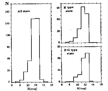 Fig. 1a-c. Distribution of stars according to the B magnitnde (all stars, F - G type and
K type stars respectively). The sharp edges at the right side of the diagrams are due to the
magnitude limit of our sample.
Based on these calibrations we determined the photometric colours of the program
stars using the Cuffey type iris photometer of the Konkoly Observatory. We measured
5 plates in UBV and 3 plates in the R and G colours. The corresponding accuracy
of photometric magnitudes obtained in this way are +-0.07, +-0.06, +-0.05, +-0.08 and
+-0.06 magnitudes for U, B, V, R and G respectively. The photometric data of our
program stars in the international system are summarized in Table 6.
2.2 Spectral classification
The spectra obtained by the 5 degree prism were classified visually using the
criteria of the Bonner Spectral Atlas (Seitter 1975). According to the sharpness of
the criteria we can define the following normal groups (a concept introduced in Mor-
gan 1951) to assign those stars which are indistinguishable from each other in respect
of the given criteria and dispersion of spectra. Considering the resolving power of our
5 degree prism and the widening of our spectra we can set up the following groups:
F8, G0, G2, G5, G8, K0, K2, K5, M0, M5.
We used the following general features in our work: Balmer lines decrease with
advancing spectral type and disappear around K0. The spectral pattern is dominated
by the CaII(H) and (K) lines, G-band and strong absorption in the region lambda4118-4216
in the blue part of the spectrum. The CaI4227 increases rapidly with advancing
spectral type after the K0. Blend MnI, FeI, SrII lambda4031- 4078 becomes increasingly
strong with advancing spectral type and is the dominating feature in the blue spectral
region of stars later than G5 and luminosity classes V. TiO bands appear around M0
and increase towards later types. lambda4215 - 4227 is intense and lambda4200, 4176, 4155 bands
are noticeable in spectral type K at luminosity class III. The characteristic features of
spectral groups are listed in Table 2. We have based our further discussion on these
subgroups supplemented with multicolour data.
3. INTERSTELLAR REDDENING
Before entering into the details of the space distribution of stars of different
spectral characteristics based on photometric parallax, we have to remove the effect of
interstellar reddening from the photometric data. Spectral classification of small scale
spectra enables us in principle to estimate the intrinsic colours of the stars and compare
them with those actually measured. In the case of stars of F8 and later, however, one
encounters difficulties. The reddening path of late-type stars on the B - V, U - B and
G - R, U - G two-colour diagrams makes a much smaller angle to the unreddened
branch of Population I stars in these diagrams, unlike stars of A5-F5 spectral types
(see the model calculations of Buser 1978a). As a consequence, even small errors in
the spectral classification could cause serious bias in determining the colour excesses
in this way. An additional difficulty arises from the photometric effect of differences in
chemical abundances. The blanketing effect, i.e. the photometric differences of stars
due to their metal abundances, can become quite prominent among spectral types of
F5 and later, especially at higher galactic latitudes. The blanketing shifts the stars
to the right and upwards on the two-colour diagrams. Both the reddening and the
blanketing shift the stars rightwards on the two-colour diagrams but in the U - B or
U - G direction, on the contrary, the results of these two effects are just the opposite:
the reddening shifts downwards while the blanketing shifts upwards. If one knows the
spectral type, therefore, one can in principle distinguish between these two effects. In
reality, however, due to the uncertainty of spectral types of G-K stars on our small
scale spectra, one encounters difficulties when trying to separate the blanketing from
the reddening in this way. To study the distribution of absorbing material responsible
for the interstellar reddening in this field, we therefore have to invoke the results of
other investigations as well. The overall galactic optical absorption due to interstellar
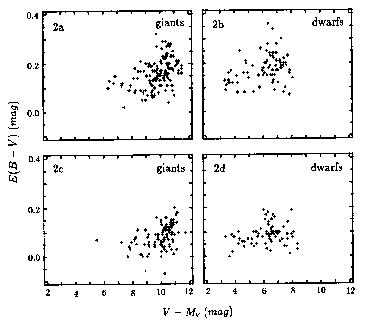 Fig. 2.a-d Plot of the E(B-V) colour excesses of the program stars, estimated by factor
analysis, versus uncorrected distance moduli. (a-b: below and c-d: above the 425th line in the
PL113 IRAS Sky Flux map). Note the similarity between the distribution of colour excesses
of giants and dwarfs indicating the presence of a nearby obscuring cloud.
dust was studied by FitzGerald (1968) and Neckel and Klare (1980). The spatial
resolution of their studies was fairly poor owing to the sparseness of stars in our 19.5
sq. degree field. Nevertheless, their studies indicated that the surface density of the
absorbing material was non-uniform, i.e it was mostly concentrated in the smaller
galactic latitude side of our field; and both studies showed an abrupt increase in
the absorption within 200 pc, revealing the presence of a nearby absorbing cloud.
These results were confirmed by our previous study on the distribution of stars of
types F7 and earlier based on 427 stars (Paparo and Balazs 1982). To get a more
detailed picture of the distribution of absorbing material in our field we invoked the
relevant IRAS Sky Flux Map. To compare the IRAS colours with our photometric
data we sampled the 100 micrometer map of the PL113 plate at the positions of our program
stars. Since the 100 micrometer radiation originates predominantly from the galactic dust
clouds (Hauser et al. 1984) and the IRAS fluxes represent the total column density
of the emitting material, we may expect good correlation with the optical absorption
only with stars which are lying behind the absorbing material in the line of sight.
The dust particles emitting the IRAS fluxes and those responsible for the optical
absorption are not necessarily identical. Furthermore, the dust clouds may differ in
their characteristic temperatures causing different infrared properties without affecting
the optical properties of the absorbing material. All these effects work against a close
correlation between the optical absorption and the measurable FIR radiation of the
dust clouds. Our expectation is therefore only justified when the distribution of dust
particles responsible for the infrared radiation is similar to the distribution of those
making the optical absorption and there are no big differences in the temperatures of
dust clouds in our area. A further difficulty arose from the influence of the Zodiacal
Light dominating the 12 micrometer and 25 micrometer radiation in our field. It was an unfortunate
circumstance that the general trend of the Zodiacal emission nearly corresponded to
those of the interstellar reddening in our case. We cannot exclude the possibility that
the correlation between the optical obscuration and the FIR might originates from this
coincidence. Nevertheless, a comparison between the optical measures of absorption
and the intensity of the FIR radiation may also have some significance.
To obtain a reliable measure for the optical absorption we tried to concentrate
in one variable all the information our photometric data contained in respect of in-
terstellar absorption. As we mentioned earlier in this paper the interstellar reddening
shifts the stars rightwards to the unreddened loci of objects on the B - V, U - B and
G - R, U - G two-colour diagrams. The orthogonal distance from the unreddened
two-colour line due to this shift, depends on the spectral type and the actual functional
form of the line joining the unreddened loci of objects in these diagrams. In the case
of Population I objects this functional form is well approximated by straight lines in
the following spectral ranges, based on the calibration of Buser (1978a):
- in the F8-K0 spectral range the loci of dwarfs and G5-G8 giants essentially
define the same straight line on the two-colour diagrams within the accuracy of
our photometric data;
- in the K0-M0 domain, in contrast, the giants and dwarfs populate different lines;
- in the M1 and M6 domain the giants are well approximated by a straight line
but both the photometric measurements and calibrations are rather uncertain
because of the increasing dominance of molecular bands in this range. We as-
signed to all of these stars the spectral type M5 in our sample. Because of the
great uncertainties in their photometric data we omitted them from the further
analysis.
Assuming that the real functional form can be well represented by these straight lines
and, furthermore letting B - V, U - B, G - R and U - G be the respective measured
colour indices in the UBV and RGU systems, then the orthogonal displacements of
stars from the unreddened Population I two-colour lines can be written in the form of
the equations:
DUBV = alpha_1*(B - V) + beta_1*(U - B) + gamma_1
DRGU = alpha_2*(G - R) + beta_2*(U - G) + gamma_2
The following table summarizes the value of coefficients in these equations, in the
spectral ranges mentioned above.
Table 3.
alpha_1 beta_1 gamma_1 alpha_2 beta_2 gamma_2
F8-K0 dwarf +0.839 -0.543 -0.444 +0.815 -0.578 -0.006
K2-M0 dwarf +0.761 -0.648 -0.202 +0.773 -0.634 +0.304
K0-M0 giant +0.875 -0.481 -0.418 +0.869 -0.495 -0.039
These displacements may not only be due to interstellar reddening but may be
partly accounted for by the blanketing effect. To get more information on these two
physical quantities and to study their influence on the measured colours separately
and in more detail, we subtracted the respective colour indices estimated on the basis
of the spectral types of our program stars from the actually measured colour indices,
i.e.:
EUB = (U - B) - (U - B)_0 , EUG = (U - G) - (U - G)_0
EBV = (B - V) - (B - V)_0 , EGR = (G - R) - (G - R)_0
The '0' indices denote Buser's normalized synthetic colours corresponding to the unred-
dened Population I values of the spectral types of our program stars. Although all of
these quantities have some relevance in measuring the amount of optical absorption,
we omitted from our further study the short wavelength colour differences, i.e. EUB
and EUG, because blanketing affects them much more seriously; as it does the possible
uncertainties that may be present in the spectral classification.
To concentrate the photometric effect of interstellar absorption into one variable
we proceeded to estimate its effect contained in EBV, EGR, DUBV and DRGU. To
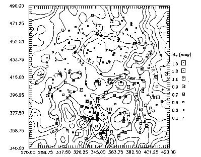 Fig. 3. Comparison of the 100 micron IRAS flux with the estimated visual absorption.
Sizes of squares are proportional to the measure of visual absorption at the place of program
stars. Both the 100 micron flux and the optical absorption are stronger in the southern part
of our field. The numbers at the left side and the bottom of the figure refer to the lines and
columns in the PL113 IRAS Sky Flux Map.
carry out this procedure we invoked a standard technique of multivariate mathematical
statistics, factor analysis. According to the basic assumption of factor analysis we
suppose that the components of an X observable m-dimensional statistical variable
can be well represented by the linear combination of k other variables, called factors.
This means
X_j = sum_{l=1}^k c_{jl} f_l + e_j, j = 1,...m & k < m
where c, f and e are the factor coefficients (loadings), factor values (scores) and
individual factors, respectively. There are a wide variety of methods published in the
literature for estimating the different components of factor models. We used the
solution based on principal components analysis (for further details on this method
see Murtagh and Heck 1987). The factors obtained by principal components analysis
are always uncorrelated. We have identified the components of X with EBV, EGR,
DUBV and DRGU and therefore m = 4 in our case.
Performing factor analysis on our data field we got a set of uncorrelated vari-
ables describing the basic dependences between the variables observed. We made the
assumption that there were some physical variables (interstellar reddening and blan-
keting in our particular case) behind the observed ones and that they determined
the variables actually observed. If the transformation between this physical variables
and those observed were linear we might expect some linear connection between the
physical and factor variables as well.
The number of significant factor variables set an upper limit for the number of
physical variables one can recognize in the given data field. To ensure the validity
of the required linearity we performed the factor analysis in the spectral groups de-
fined above, separately. According to the principal components analysis technique
the variables measured were represented by linear combinations of eigen vectors of
the correlation matrix of the variables observed. Factor analysis then proceeded by
dropping eigenvectors with small eigenvalues and assumed only those to be significant
which were above a certain threshold. In the SPSS software package what we used
in computing the factor model, the default value of this threshold was set to equal 1.
Table 4. summarizes the eigenvectors of the correlation matrix in the case of the F-G
dwarfs and the K giants separately:
Table 4.
F-G dwarfs K giants
factor eigenvalue cum.pct. eigenvalue cum.pct.
1 2.898 72.4 2.566 64.2
2 .860 93.9 .810 84.4
3 .213 99.3 .592 99.2
4 .029 100.0 .032 100.0
Examining Table 4. one can infer that in both cases there is only one eigenvalue lying
above the default threshold. The second eigenvalues, however, are close to unity and
we tried to reproduce the covariance matrix keeping these factor variables. In the case
of the dwarf stars the use of these two factors gave satisfactory reproduction of the
covariance matrix. In the case of giants this reproduction was not so good but was
still acceptable. We therefore used these two factors in our further calculations.
There are no clear rules concerning the making of comparisons between the vari-
ables obtained by factor analysis and those representing real physical quantities. Since
the 100 micron IRAS fluxes are good measures of the amount of galactic dust, we iden-
tified those factor variables with interstellar absorption which showed the maximum
correlation between the intensity of FIR radiation and the factor values given by the
analysis. We expected correlation between the optical measure of absorption and the
100 micron flux only with those stars which are lying at greater distances than the bulk
of emitting dust material responsible for the FIR radiation and detected by the IRAS
mission.
3.2 Distribution of the absorbing material
We plotted the estimated colour excesses against the distance modulus of the
stars in our sample in Fig. 2a-d for giants and dwarfs separately. We divided the whole
field by the 425. line of the respective IRAS Sky Flux map in order to demonstrate
the assimmetry in the surface distribution of the obscuring material over the whole
area. It was also apparent on these plots that there were no significant difference
between the distributions of the optical absorption of dwarfs and giants. Furthermore,
the absorption of dwarfs increased up to 0.7 mag near to 6.7 of uncorrected distance
modulus and did not change remarkably among the giants. It means that the vast
majority of the absorbing material was concentrated within the distance modulus near
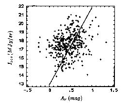 Fig. 4. Correlation between 100 micron IRAS flux and the estimated visual absorption. A
line with 9 MJy/Sr per magnitude slope, found by de Vries and Le Poole (1985) for some
high latitude dust clouds is also indicated.
to 6 corresponding to a distance of about 150 pc. We might therefore expect correlation
between the IRAS fluxes and the stellar reddening with those stars which were lying
behind this distance. The surface distribution of absorbing material was not uniform
in this area, as was suggested by the earlier investigations. The patchy structure
of the interstellar dust is also apparent on the IRAS Sky Flux maps. We plotted
the reddening data of stars of r > 150 pc, represented in Fig. 3, in order to make a
comparison between the surface distribution of the optical absorbing material and the
FIR radiation. By doing this we recovered the results of the earlier investigations but
with better angular resolution.
To get reliable correlation between the optical and infrared data we divided the
stars in our sample into three groups: dwarfs r < 150 pc (V - M_V < 6.7), dwarfs
r > 150 pc and giants. Table 5. shows the correlations between the factor values and
the 100 micron flux within each of these groups:
Table 5.
dwarfs1 dwarfs2 giants
Flux. f1 f2 Flux. f1 f2 Flux. f1 f2
Flux.(100) 1.00 .06 -.07 1.00 .33* .18 1.00 .25** -.03
f1 .06 1.00 .07 .33* 1.00 .01 .25** 1.00 .00
f2 -.07 .07 1.00 .18 .01 1.00 -.03 .00 1.00
number of cases: 91 52 204
1-tailed Signif: * - 0.01 ** - 0.001
Examining this table one can clearly see that factor f1 has significant correlation with
the FIR radiation in two of the groups, whereas f2 has not. The lack of significance
in the first group and the significance in the second and third ones reflect the fact that
the optical absorption, and also the FIR radiation, originate from a nearby dust cloud.
Fig. 4 summarizes the dependence of the optical absorption measures on the 100 micron
radiation. We computed a best fitting line to the points in this figure by extracting the
common factor in A_v and 100 micron flux. The shape of this line was 5.4 MJy/Sr/mag
while de Vries and Le Poole (1985) obtained 9 MJy/Sr/mag for some high latitude
extended dust clouds. We adopted the estimated value of f1 as a measure of the optical
absorption and converted it into factor-analysis-predicted EBV and EGR using the
linear relation between the colour excesses and the factor values. The measure of the
optical absorption can be obtained using the standard relationship between selective
and total absorption. We used here the coefficients published by Buser (1978a).
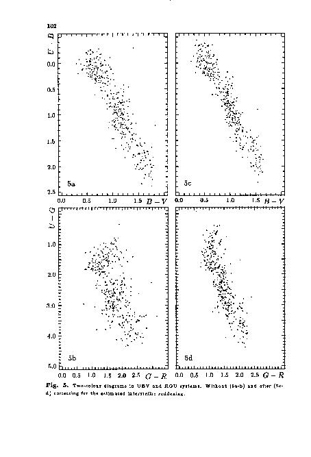 Fig. 5. Two-colour diagrams in UBV and RGU systems. Without (5a-b) and after (5c-
d) correcting for the estimated interstellar reddening.
4. SPATIAL DISTRIBUTION OF THE STARS
4.1 Generalization of the convolution equation for multivariate case
After eliminating the effect of the interstellar reddening we could proceed to
the determination of the spatial distribution of our stars. To check the reliability of
the procedure we used for the elimination of reddening from our data we compared
the two-colour diagrams of the non-corrected colour indices with those corrected us-
ing the method described in the previous paragraph. The power of this procedure is
demonstrated in Fig. 5. To derive the space densities of our stars we made the usual
assumption that their true absolute magnitudes are represented by a Gaussian ran-
dom variable with a mean value given by their spectral type, luminosity class, chemical
composition and a standard deviation (McCuskey 1966). We have a multicolour sam-
ple in our case and consequently the absolute magnitude itself is also a multivariate
Gaussian random variable with a mean according to the spectral characteristics of the
stars and a Summa covariance matrix. We have omitted from the further calculations the
U colour because, as we pointed out in the previous paragraph, the errors inherent in
spectral classification affect this spectral band most seriously. Let
Phi(M|Sp) = {exp (-(M - M0)^T Sigma_{-1} (M - M0)) / (2pi)^{m/2} DET(Sigma)}
a multivariate Gaussian where M represents the set of variables B, V, R and G (so
we have a four dimensional variable in our case); Sp the spectral type given, M0 the
mean value of absolute magnitude and Summa the covariance matrix. With these notations
we can generalize the standard integral equation of stellar statistics (Kurth 1967) in
the form of
A(m|Sp) = int_{-infty}^{+infty}Delta(rho)Phi(m - rho | Sp)dp
Where m and rho are multivariate random variables representing the apparent magni-
tudes and distance modulus in different colour bands while A and Delta stand for their
probability densities respectively. To solve this integral equation we approximated the
integral expression with a sum of
A(m|Sp) = sum_{l=1}^k q_l Phi(m - rho_l | Sp), l = 1,...,k
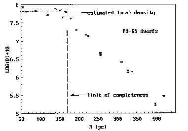 Fig. 6a. Dependence of logarithmic density on the distance in line of sight in case of F8-G5
dwarfs. The limit of completeness of our sample is marked by a vertical dashed line.
containing $q_l = Delta(rho_l)drho$ and $rho_l$ as unknown parameters to be determined. To estimate
the set of the unknown parameters we used the maximum likelihood method. We
defined the maximum likelihood function in the usual way:
L(a) = sum_{i=1}^nlogA(m_i | Sp).
In this equation a represents the set of parameters to be estimated and n the size of
the sample. The maximum likelihood principle requires the estimation of those values
of a which maximize L(a), i.e.:
{partial L(a) / partial a} = 0 .
The derivatives of L(a) yielded a system of equations and the solution of this system
resulted in the parameter values we were looking for. In the following we discuss the
results of these computations in separate spectral subgroups.
4.2 F8-G5 stars
The F8 - G8 stars formed a separate group in our two-colour diagrams. After
being corrected for interstellar reddening they satisfactorily concentrated along the
unreddened main sequence line in the two-colour diagrams. We cannot distinguish
among the subdwarfs, dwarfs, subgiants and giants in this spectral region using our
small scale spectra. Using larger dispersion spectra for a magnitude limited sample,
Kharadze et al. (1989) concluded that among their G type stars there were practically
the same numbers of subgiants and dwarfs. On the other hand, in Houk's (1983) HR
diagram based on the Michigan spectral survey data, the stars mainly populated the
main sequence in the F8 - G5 region. Kharadze et al. assigned all stars to subgiants
which could not be classified as either giant or dwarf. Their number of subgiants may
therefore perhaps have been overestimated. We made the assumption in our further
analysis that the vast majority of our F8 - G5 stars belonged to the main sequence
dwarfs.
As a result of the reddening correction a small number of the stars were shifted
above the main sequence line. Their corrected position corresponded to those produced
by the blanketing effect. The shift gave an ultraviolet excess of about 0.2 mag in the
UBV and 0.3 mag in the RGU system and might be explained by metal deficiency
in these stars. Measurements using a more sophisticated photometric system such as
the Stromgren uvby photometry could prove the validity of this conclusion. With the
exception of these UV objects we assumed that the F - G stars were main sequence
stars in our sample and assigned to them absolute magnitudes according to their
spectral types given by Allen (1973).
The absolute magnitude increases very rapidly within this spectral group. From
the value of 4.0 at F8 stars it reaches 5.5 at G8 in the V band. Since our sample
was magnitude limited the limiting distance in our sample, i.e. the distance which
the space densities were biased beyond, varied strongly from F8 to G8 as well. To
get a greater limiting distance but still enough objects to make statistical studies we
restricted ourselves to the spectral range of F8 - G5.
Performing the maximum likelihood algorithm outlined above we obtained an
estimation of the space densities as a function of the distances from the Sun. Fig. 6a
shows the logarithm of these densities as a function of the distances. The limit of
completeness is also indicated. The points obtained run nearly horizontally in the
unbiased range of the diagram. Since the limiting distance is about 250 pc in our case,
the distance from the galactic plane is less than 70 pc in the unbiased range. This
means that we are practically seeing the space density of F8 - G5 stars in the galactic
plane.
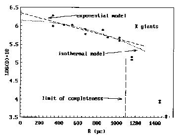 Fig. 6b. Dependence of logarithmic density on the distance in line of sight in case of K
giants. The limit of completeness of our sample is marked by a vertical dashed line. Our fits
with an isothermal and an exponentional model are also indicated.
4.3 K giants
The separation of K giants from the dwarfs is in principle possible on our small
scale spectra. In practice, however, we succeeded in doing it with satisfactory reliability
only with stars having well exposed spectra on our plates, i.e. with the brighter stars in
our sample. Most of these stars appeared to be giants which nicely followed the line of
the Population I giants on the two-colour diagrams after being corrected for reddening.
The majority of fainter stars not bright enough for reliable luminosity class estimation
also concentrated along the Population I giant line. In some cases, however, we had
stars departing significantly from this line. In a considerable number of these cases the
photometric images of objects in one of the colours distorted by a neighbouring star or
the U colour was too faint for reliable brightness determination. Of course, we could
not exclude the possibility that some of them were dwarfs, especially those lying along
the dwarf line, or metal poor giants, if their positions on the two-colour diagram were
realistic. Again, more accurate photometric or spectroscopic measurements would be
desirable in these cases. We also omitted from the further analysis the stars with
spectral types later than M0. We rejected 35 stars altogether in this way. Assuming
that the stars remaining in the sample were Population I giants we assigned absolute
magnitudes to them as given by Allen (1973). The space densities yielded by the
maximum likelihood algorithm are displayed in Fig. 6b.
The main aim of our studying the space densities in this low latitude field was to
compare spatial distributions in the galactic caps with those obtained in the present
investigation. In particular, we were interested in testing the plane-parallel hypothesis,
i.e. the hypothesis that the low latitude distributions can be well approximated by
the substitution of z = r*sin(b) into D(z), the density in the direction of the polar
caps, due to the high flattening of the galactic disc. The most extensive study in
the direction of the North Polar Cap was the work of Upgren (1962) containing 4027
stars of spectral class G5 and later in a 396 square degree field down to a limiting
photographic magnitude of 13.0. We tested this hypothesis by substituting z = r*sin(b)
(b = +16.5 deg in our case) into Upgren's density data and converted them into the
distribution of the distance moduli which was the output of our maximum likelihood
algorithm. The result of this comparison is shown in Fig. 7. This figure demonstrated
with satisfactory significance that our points followed Upgren's transformed curve up
to a distance modulus of 10 mag corresponding to the limit of completeness in our
sample. It has also been demonstrated that the plane-parallel approximation holds
at least up to 1000 pc from the Sun in this direction.
In Fig. 6b we have shown the logarithmic space density of K giants of our sample
as a function of the distance in the line of sight. The usual assumption that the space
density is well approximated by an exponential function with a scale height depending
on the absolute magnitude (see e.g. Bahcall and Soneira 1980) would result in a
straight line in this figure. The scale height of the best fitting line corresponded to
200 pc perpendicular to the galactic plane. Assuming an isothermal model, on the
other hand, we get
log D(z) - log D(0) = -{u(z) / sigma_W^2}
where the gravitational potential u(z) is well approximated by
u(z) approx u(0) - {u(0)`` / 2}z^2
near to the galactic plane. This analytical form of the logarithmic density also fits
satisfactorily with our data.
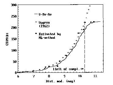 Fig. 7. The cumulative space density of K-type stars plotted against distance moduli for
our program stars (full line) and for Upgren's (1962) data (crosses) after z = r*sin(b)
scaling. Departure from Upgren's data above 10 magnitude is due to the incompleteness of
our sample in that range.
5. CONCLUSIONS
We have investigated 424 stars of spectral types of F8 and later in a 19.5 sq.
degree field around IC 4665. The main purpose of our study was to make comparisons
between the space densities of late-type stars in the galactic caps with samples taken
from fields at great angular distances from the poles (6 = +16.5 deg in our case). In
particular, we were interested in testing the plane-parallel hypothesis of the density
distribution, i.e. the hypothesis that the spatial density of the Population I stars
observed at great angular distances from the galactic caps is well approximated by the
z = r*sin(b) scaling of the distributions obtained in the polar regions.
The major difficulty in making the comparison between our field and the polar
region is the adequate treatment of the patchy distribution of the interstellar obscuring
material over the field investigated and its elimination from the photometric data. To
get an adequate estimation of the effect of the absorption we joined the power of
the UBV and RGU photometric systems combined with the results of classification
on small scale spectra. These data enabled us to get E(B - V), E(G - R) and
perpendicular distances from the unreddened loci of the Population I stars in the two-
colour diagrams, DUBV and DRGU. We used the factor analysis of multivariate
mathematical statistics in order to extract the effect of absorption from the data
field defined by EBV, EGR, DUBV and DRGU. To identify the factor component
corresponding to the interstellar reddening we invoked the corresponding IRAS Sky
Flux Data. After removing the interstellar reddening from our photometric data we
computed the spatial densities for the F8 - G5 dwarfs and the K giants separately.
We used a maximum likelihood algorithm for obtaining the space densities from the
photometric data. We can summarize the main conclusions of our paper as follows:
1. A significant amount of the absorbing material concentrates closer than 150 pc
in our area producing A_V = 1 mag at the densest part of the obscuring cloud.
2. There is a weak but still significant correlation between the optical measures of
absorption and the IRAS 100 micron Sky Flux Maps data. The shape of the best
fitting line between A_V and 100 micron flux equalled 5.4 MJy/Sr/mag.
3. The spatial densities of F8 - G5 dwarfs essentially reflect the densities obtained
in the galactic plane. In a few cases UV excess seems to be present but this needs
further confirmation based on measurements in more sophisticated photometric
systems.
4. The distribution of distance moduli of K giants in our sample can be well mod-
elled by the z = r*sin(b) scaling of Upgren's data from the North Polar region.
The actual form of the space density curve of the K giants can be fitted by an
exponential distribution with a scale height of 200 pc perpendicular to the galac-
tic plane. A satisfactory fit can also be obtained by an isothermal model which
is more realistic from the physical point of view. While the exponential model
predicts a discontinuity in the density gradient at z = 0, the isothermal version
moves through this point with continuous derivative.
ACKNOWLEDGEMENTS
We are indebted to Dr. M. Kun for her useful advice in recognizing the K giants
on our small scale spectra. We wish to thank Dr. K. Ishida (University of Tokyo)
and Dr. L. Szabados for reading the manuscript and making valuable comments. We
are also grateful to Mr. Holl for his kind help in picture processing the IRAS Sky
Flux Maps and to Dr. J. Kelemen for his contribution in making the identification
map. The kind permission for the relevant IRAS data by the Huyghens Laboratory, in
particular the help of Prof. H.J. Habing and Dr. E. Deul, is also acknowledged.
Budapest - Szabadsaghegy, Dec 20, 1990.
References:
Alcaino, G., 1965, Bull. Lowell Obs., 6, No.7, 167.
Allen, C. W., 1973, Astrophysical Quantities 3rd. ed., Athlona Press, London.
Bahcall, J. N., 1984, Astrophys. J., 276, 169. (1984ApJ...276..169B)
Bahcall, J. N., Soneira, R. M., 1980, Astrophys. J., Suppl. Ser., 44, 73. (1980ApJS...44...73B)
Balazs, L. G., 1975, Mitt. Sternwarte Ung. Ak. Wiss. 68. CoKon 68
Balazs, L. G., 1977, The Cosmogonical Significance of the z Distribution of Stars in "Chemical and Dynamical Evolution of our Galaxy" IAU Coll. 45, 271.
Balazs, L. G., 1984, Statistics of A-type Stars as Possible Indicator of Star Formation in "Astronomy with Schmidt-Type Telescopes" ed. Capaccioli M., D. Reidel Publ.Co. p.269.
Balazs, L. G., Paparo, M., Toth, I., 1985, Mitt. Sternwarte Ung. Ak. Wiss. 85. CoKon 85
Buser, R., 1978a, Astron. Astrophys., 62, 411. (1978A&A....62..411B)
Buser, R., 1978b, Astron. Astrophys., 62, 425. (1978A&A....62..425B)
de Vries, C. P., Le Poole, R. S., 1985, Astron. Astrophys., 145, L7. (1985A&A...145L...7D)
FitzGerald, M. P., 1968, Astron. J., 73, 983. (1968AJ.....73..983F)
Hauser, M. G., Gillett, F. C., Low, F. J., Gautier, T. N., Beichman, C. A., Neugebauer, G., Aumann, H. H., Band, B., Boggess, N., Emerson, J. P., Houck, J. R., Soifer, B. T., and Walker, R. G., 1984, Astrophys. J., 278, L15. (1984ApJ...278L..15H)
Houk, N., 1983, The Nearby Stars and the Stellar Luminosity Function, IAU Coll. No. 67, Ed. by Philip A. G. D. and Upgren A. R., L. Davis Press p.345.
Kharadze, E. K., Bartaya, R. A., Dluzhnevskaya, O. B., Piskunov, A. E., Pavlovskaya, E. D., 1989, Astrophys. Space Sci., 151, 319. (1989Ap&SS.151..319K)
Kurth, R., 1967, Introduction to Stellar Statistics, Pergamon Press, Oxford.
McCuskey, S. W. 1966, Vistas in Astronomy, 7, 141.
Morgan, W. W., 1951, Publ. Univ. Michigan Obs., 10, 33.
Murtagh, F., Heck, A., 1987, Multivariate Data Analysis, Astrophys. Space Sci. Lib., 131. D. Reidel Publ.Co.
Neckel, T., Klare, G., 1980, Astron. Astrophys., Suppl. Ser., 42, 251. (1980A&AS...42..251N)
Paparo, M., Balazs, L. G., 1982, Mitt. Sternwarte Ung. Ak. Wiss. 82. CoKon 82
Seitter, W. C., 1975, Atlas for Objective Prism Spectra; Bonner Spectral Atlas II., Ferd. Dummler Verlag, Bonn.
Steinlin, U. W., 1968, Zeitschrift fur Astrophysik, 69, 276.
Upgren, A. R., 1962, Astron. J., 67, 37. (1962AJ.....67...37U)
Woolley, R., Stewart, J. M., 1967, Mon. Not. R. Astr. Soc., 136, 329. (1967MNRAS.136..329W)
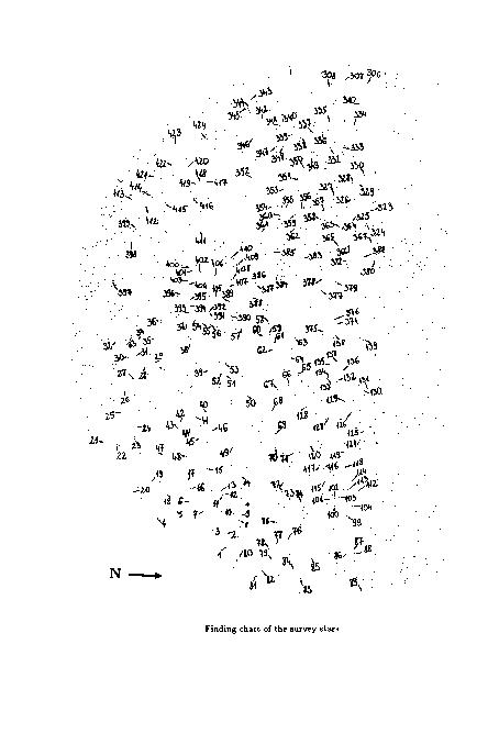 Finding chart of the survey stars
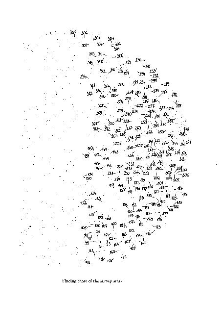 Finding chart of the survey stars
Table 6. (Spectra and photometric data of survey stars) No. Sp. V B-V U-B G G-R U-G remarks 1 G5 III 7.04 0.87 0.41 7.54 1.44 1.97 2 K5: 11.39 1.62 1.74 12.59 2.59 3.35 3 K2 III 10.03 1.39 1.48 10.83 2.01 3.31 4 M5 III 10.43: 1.92: 1.39 11.87 3.24: 2.98: 5 K5 III 9.78 1.63: 1.99: 10.70 2.48 3.97 6 K2: 11.18 1.00 0.70 11.85 2.01 2.23 7 K2 III 9.68 1.47 1.59 10.44 2.08 3.55 8 G2 11.45 0.97 0.12 12.50 1.39: 1.15: early 9 K0 III 11.29 1.18 0.77 12.06 2.09 2.35 10 G2 11.40 0.92 0.04 11.91: 1.78: 1.57: blend 11 M0 III 9.67 1.75 1.63 10.69 2.47 3.55 12 G5: 11.75 0.77 0.01 12.22 1.55 1.45 13 K5 III 8.01 1.58 2.05 8.92 2.26 4.01 14 G8 9.72 0.78 0.35 10.06 1.27 1.99 15 K0 III 9.56 1.15 1.02 10.13 1.83 2.82 16 K2: 11.37 1.37 1.27 12.30 2.24 2.92 17 K0 III 10.77 1.18 0.72 11.51 2.01 2.33 18 G0 11.58 0.80 0.04 11.99 1.68 1.57 early 19 F8 9.74 0.53 0.10 9.84 1.34 1.74 20 K5 III 11.07 1.56 1.61 11.95 2.49 3.51 early 21 K5: 11.52: 0.39: 0.66: 11.46 1.88: 2.44: edge 22 G2 10.85 0.87 0.04 11.32 1.56: 1.56: early 23 K5 III 9.63 1.74 2.02 10.60 2.61 4.04 24 M0 III 10.67 1.78 1.82 11.56 2.53 3.91 25 K2 III 10.95 1.41 1.37: 11.71 2.41: 3.24: 26 K2 11.14 1.40 0.93 11.85 2.40 2.77 27 K2 III 8.82 1.53 1.55 9.58 2.18 3.54 28 M0 III 10.34 1.64 1.83 11.15 2.44 3.91 29 M0: 10.89 1.74 2.10 11.93 2.70 4.06 30 G8 III 11.19 1.07 0.61 11.73 1.85: 2.32 31 M0 III 9.76 1.82 1.21 10.53 2.72 3.36 32 K0: 11.00 1.16 0.50: 11.59 2.00: 2.21: 33 K0 III 10.56 1.16 0.79 11.10 2.04 2.59 34 K0 III 11.13 1.23 0.76 11.87 2.30: 2.41: 35 K0 10.82 0.96 0.53 11.30 1.84 2.19 36 K0 III 10.49 1.10 0.80 10.97 1.94 2.61 37 K0 III 10.29 1.23 0.95 10.86 1.90 2.81 38 G5: 11.33 0.77 -0.16: 11.74: 1.69: 1.31: blend 39 K0 III 9.74 1.19 1.27 10.30 1.84 3.15 40 M0 III 10.44 1.75 2.01 11.53 2.66 3.92 41 G0: 11.01: 0.91: 0.30: 11.72: 1.75: 1.66: early 42 G8 9.63 0.91 0.36 10.11 1.56 1.95 43 K2 III 10.84 1.37 1.17 11.67 2.19 2.91 44 G0 11.68 0.77 0.02 12.08 1.58 1.54 45 G5: 11.09 0.86 0.41 11.60: 1.77: 1.95: blend 46 K2 III 9.20 1.55 1.88 10.18 2.30 3.72 47 K0 III 9.71 1.30 1.11 10.35 1.85 2.97 48 K5 10.88 1.21 1.19 11.77 2.24 2.75 49 G8 8.80 0.89 0.29 9.23 1.37 1.91 50 K5 III 9.51 1.63 1.79 10.41 2.31 3.75 Table 6. (Continued) No. Sp. V B-V U-B G G-R U-G remarks 51 K2 III 10.67 1.38 1.46 11.63 2.28 3.12 52 K5 10.91 1.27 0.94 11.62 1.92 2.68 53 M0 III 10.06 1.77 2.26 11.12 2.66 4.25 54 K0 III 10.78 1.11 0.77 11.27 1.74 2.57 55 K0 III 11.03 1.16 0.93 11.76 1.99 2.56 56 M5 III 11.24 1.77 1.66 12.13 2.54 3.72 57 F8 10.90 0.69 -0.22 11.26 1.34 1.24 58 F8 10.94 0.76 -0.10 11.58 1.70: 1.15: early 59 G0 11.20 0.68 -0.01 11.63 1.39 1.39 60 G5 11.11 0.81 0.28 11.67 1.53 1.71 61 F8 11.48 0.64 -0.09 12.06: 1.83: 1.13: early 62 G0 11.34 0.78 -0.02 11.89 1.67 1.34 63 G5 10.93 0.95 0.08 11.83: 1.95: 1.25: early 64 G0: 11.68 0.95 -0.10 12.33: 1.99: 1.28: blend 65 G0 11.14 0.53 -0.23 11.57 1.29: 1.02 66 G8 8.92 0.79 0.27 9.38 1.38 1.78 67 K5 III 9.20 1.79 1.98 10.24 2.51 3.96 68 K2 III 10.22 1.40 1.78 11.11 2.19 3.57 69 K2 III 10.02 1.20 1.02 10.83 1.93 2.62 70 K0: 10.62 0.80 0.68 11.13: 1.60: 2.21: 71 G0 10.68 0.67 0.23 11.23 1.56 1.55 72 K5: 10.70 1.25 1.04 11.50 1.98 2.69 73 K0 III 10.96 1.11 0.85 11.80 2.08 2.32 74 K0 III 10.08 1.16 0.99 10.84 1.92 2.61 75 K2 III 9.14 1.26 1.26 9.82 1.72 3.07 76 G8 III 9.42 1.02 0.90 9.99 1.55 2.58 77 K0 III 10.45 1.17 0.97 11.18 1.77 2.61 78 G0 11.84 0.76 0.01 12.54 1.64 1.22 79 K0 III 11.28 1.33 0.75 12.34 2.08 2.16 80 K5 III 10.12 1.61 1.72 11.30 2.42 3.38 81 K0 III 10.60 1.08 0.98 11.33 2.04 2.56 82 G2 9.97 0.88 0.16 10.45 1.54 1.70 early 83 K0 III 8.75 1.10 1.30 9.35 1.74 3.08 84 G5: 11.75 1.27 0.57: 12.57: 2.05: 2.14: 85 M0 III 10.44 1.69 1.76 11.61 2.56 3.50 86 K0 III 10.87 1.30 1.03 11.73 1.96 2.66 87 G8 III 10.21 1.10 0.68 10.83 1.66 2.33 88 K0 III 9.13 1.05 0.82 9.74 1.51 2.47 89 K2 III 11.10 1.44 1.80 11.87 2.80: 3.75: 90 K0 III 11.19 1.03 1.22 11.70 2.10: 3.01 91 G5 8.85 0.73 0.34 9.16 1.29 1.96 92 G5: 11.74 0.71 0.13 12.42: 1.79: 1.33: blend 93 G0 9.84 0.68 0.30 10.19 1.21 1.83 early 94 F8 8.87 0.56 0.17 9.00 1.04 1.81 95 G0 10.70 0.71 0.11 11.06 1.29 1.64 96 K0 III 10.62 1.03 0.84 11.16 1.57 2.54 97 K0 III 10.95 1.16 0.89 11.57 1.71 2.63 98 M0 10.67 1.47 1.11 11.63 2.32 2.78 99 G0 11.17 1.00 0.44 11.96: 1.79: 1.81: blend 100 M0 III 10.80 1.68 1.71 12.02 2.65 3.38 Table 6. (Continued) No. Sp. V B-V U-B G G-R U-G remarks 101 G8 10.84 0.75 0.38 11.35 1.33 1.83 102 G0 11.20 0.60 0.20 11.59 1.18 1.63 103 K2 III 9.60 1.22 1.38 10.30 1.33 3.17 104 M0: 10.76 1.78 0.65: 12.09: 2.71: 2.12: blend 105 K2 III 10.25 1.52 1.76 11.32 2.31 3.47 106 K2 III 10.97 1.58 1.85 11.93 2.08 3.73 107 K0 10.19 0.80 0.54 10.64 1.38 2.11 108 G2 11.22 0.74 0.25 11.79 1.55 1.61 109 F8: 11.94 0.64 -0.07 12.50 1.61 1.17 110 K5 11.24 1.21 1.11 12.19 1.92 2.60 111 K2 III 10.20 1.19 1.33 10.87 1.71 3.11 112 K2 III 9.29 1.18 1.37 10.04 1.80 3.07 113 K2 III 8.01 1.29 1.29 8.73 1.68 3.09 114 K5 10.69 1.24 1.04 11.51 1.87 2.66 115 K0 III 7.83 1.17 1.19 8.51 1.69 2.93 116 F8 11.24 0.66 0.06 11.85 1.56 1.28 117 K2 III 9.64 1.23 1.15 10.36 1.71 2.89 118 F8: 12.08 0.57 -0.02 12.60: 1.30: 1.21: 119 K2 III 11.03 1.19 1.27 11.92 1.91 2.82 120 K0 III 11.17 1.28 0.74 12.22 2.07: 2.12 121 F8 11.41 0.50 -0.03 11.83 0.95 1.25 122 G5 11.22 0.82 0.19 11.83 1.52 1.56 123 F8 9.78 0.55 -0.03 10.11 1.10 1.37 124 K0 III 10.71 1.20 1.10 11.41 1.74 2.82 125 G0 11.45 0.61 0.05 11.94 1.26 1.36 126 K0 III 10.59 1.15 1.25 11.30 1.71 2.95 127 K0 III 10.30 1.17 1.16 11.02 1.93 2.84 128 K0 III 10.98 1.18 0.98 11.87 1.99 2.48 129 G0: 11.96 0.56 -0.05: 12.36: 1.15: 1.29: 130 M0 III 8.31 1.63 2.16 9.30 2.17 4.10 131 G2 11.37 0.69 0.20 11.87 1.32 1.58 132 K0 III 8.41 1.12 1.04 9.06 1.63 2.74 133 G0 11.45 0.61 -0.22 11.90 1.46 1.08 134 G2 10.99 0.82 0.04 11.60 1.75 1.39 135 K0 III 8.96 1.19 0.82 9.68 1.72 2.47 136 G0: 11.66 0.75 -0.16 12.40: 1.47: 0.97: 137 F8 11.65 0.57 -0.08 12.37 1.65 0.94 138 K5 III 8.76 1.49 1.76 9.63 2.05 3.65 139 G8 III 10.59 0.97 0.60 11.20 1.65 2.15 140 G2 8.90 0.73 -0.06 9.23 1.03 1.48 141 K0 III 10.24 1.05 0.81 10.76 1.50 2.55 142 K5 III 8.92 1.67 1.97 9.86 2.11 3.96 143 K2 III 9.10 1.37 1.53 9.87 1.85 3.38 144 F8 10.37 0.54 0.04 10.59 1.12 1.55 early 145 K2 III 10.63 1.21 1.35 11.43 1.76 3.02 146 K2 III 10.18 1.49 1.60 10.90 1.91 3.61 147 F8 11.69 0.49 -0.07 12.34 1.40 0.96 early 148 G8 III 7.80 0.96 0.84 8.32 1.42 2.51 149 G5 11.20 0.67 0.29 11.54 0.98 1.83 150 M5 III 10.95 1.74 1.07 12.16 2.55 2.70 Table 6. (Continued) No. Sp. V B-V U-B G G-R U-G remarks 151 F8 12.35 0.29 0.01 12.53 1.22 1.37 152 G8 III 9.84 1.03 0.70 10.08 1.34 2.51 153 K0 III 10.86 1.19 0.97 11.85 1.74 2.58 154 K5 III 10.00 1.50 1.75 10.80 1.98 3.71 155 K5 III 10.55 1.73 1.98 11.32 2.01 4.16 156 K2 III 11.90 1.31 1.10 12.67: 1.55: 2.84: early 157 F8 12.33 0.38 0.02 12.69 0.79: 1.27 early 158 K0 III 10.78 1.20 1.09 11.35 1.55 2.92 159 K0 III 11.56 1.22 0.43 12.10 1.44 2.22 160 G5 9.72 0.84 0.30 10.03 1.11 1.85 161 K0 III 10.67 1.16 1.22 11.33 1.69 2.97 162 K0 III 11.13 1.09 1.01 11.76: 1.68: 2.70: 163 G5 10.66 0.71 0.27 10.91 1.16 1.92 164 G8 III 8.89 0.94 0.85 9.30 1.41 2.82 165 K0 III 5.99 1.05 1.29: 6.51 1.72 3.10: HR6590 166 M0 III 9.88 1.52 1.75 10.89 2.53 3.51 167 G0 10.71 0.61 0.05 10.88 1.12 1.67 168 K2 III 10.24 1.38 1.39 10.86 1.86 3.38 169 G0 10.68 0.81 0.09 11.78: 1.75: 0.79: early 170 K5 III 11.01 1.62 1.55 11.66 2.01 3.72 171 G5 11.29 0.75 0.30 11.59 1.14 1.95 172 K5 III 10.01 1.54 1.93 l0.88 1.98 4.10 173 K0 III 10.87 1.15 1.06 11.42 1.75 2.89 174 K2 III 10.72 1.21 1.00 11.26 1.53 2.87 175 K2 III 10.97 1.33 1.34 11.69: 1.70: 3.18: 176 K0 III 10.46 1.18 1.20 10.80 1.34: 3.27 177 G2 12.24 1.09 0.41 12.88: 1.47: 2.20: 178 G0 11.96 0.54 0.21 12.26: 0.91: 1.87: 179 G2 11.11 0.75 0.28 11.50: 0.83: 1.83: 180 K0 III 8.61 1.22 1.27 9.19 1.35: 3.18 181 G0 11.28 0.64 -0.01 11.45 1.05 1.60 early 182 G8 III 10.22 1.01 0.86 10.51 1.48 2.57 183 G5 10.73 0.70 0.17 10.75 1.26 2.03 edge 184 K0 III 10.28 1.14 0.89: 10.36 1.41 3.15: edge 185 K2 III 9.76 1.19 1.24 10.06 1.71 3.37 186 K0 III 11.62 1.11 0.91 12.06 1.83 2.79 187 F8 10.94 0.60 -0.06 10.90 0.88 1.75 early 188 G2 10.90 0.50 0.19 10.95 1.03 1.87 189 F8 10.32 0.88 -0.09 10.45 1.11 1.61 190 G8 III 11.35 0.90 0.85 11.83 1.74 2.28 191 G8 III 11.74 1.22 0.58 12.33 1.72 2.32 192 M5 10.87 1.57 1.57 12.14: 2.94: 3.09: 193 G0 8.62 0.60 0.24 8.92 0.91 1.76 194 M5 III 11.27 1.71 0.97 12.44 2.54 2.80 195 G5 8.40 0.84 0.70 8.83 1.28 2.35 196 K0 III 10.05 1.07 1.28 10.51 1.50 3.15 197 K0 III 11.37 1.28 1.11 11.99 1.70 2.96 198 K2 III 10.99 1.28 1.38 11.70 1.87 3.19 199 M0 III 9.75 1.81 2.23 10.71 2.32 4.19 200 K2 III 10.93 1.15 1.36 11.59 1.58 3.12 Table 6. (Continued) No. Sp. V B-V U-B G G-R U-G remarks 201 G2: 11.97 0.53 0.26 12.29 1.33 1.71 202 G0 11.10 0.61 0.17 11.33 1.18 1.75 203 F8 11.45 0.42 0.11 11.51 1.04 1.71 204 F8: 12.00 0.49 0.11 12.09 1.22: 1.73 205 G0: 12.06 0.57 0.02 11.98 1.17 1.86 206 G8 III 11.45 0.96 0.77 11.62 1.47 2.78 207 G8 10.78 0.72 0.38: 10.75 1.13 2.35: 208 K0 III 11.24 1.21 1.19 11.56 1.74 3.31 209 K0 III 10.59 1.04 1.24 10.79 1.56 3.36 210 K0 III 10.89 1.05 1.07 11.35 1.72 2.91 211 G8 9.09 0.65 0.62 9.20 1.15 2.43 212 K0 III 10.73 0.99 1.46: 10.71: 1.16: 3.79: edge 213 K0 III 10.48 0.93 1.15 10.56 1.48 3.29 214 G8 III 11.49 0.94 0.70 11.30: 1.10: 3.04: 215 K0 III 10.01 1.03 0.95 10.22 1.48 3.00 216 K0 III 10.48 0.99 1.12 10.87 1.68 2.99 217 K2 III 11.15 1.19 1.20 11.78: 1.80: 3.00: 218 F8: 12.08 0.44 0.18 12.18 1.65: 1.76 219 G5 11.00 0.60 0.31 11.24 1.43: 1.90 220 K0 III 10.51 0.99 1.20 10.91 1.49 3.08 221 K0 III 11.05 1.17 1.06 11.63 1.65 2.88 222 K5 III 10.90 1.43 1.97 11.66 2.20 3.95 223 K2 III 8.77 1.21 1.67 9.31 1.60 3.65 224 G0 11.41 0.51 -0.17 11.83 1.08 1.09 225 G2: 11.83 0.61 0.04 12.05 0.91 1.61 226 F8: 11.95 0.45 0.04 12.24 1.27 1.42 227 K2 III 10.97 1.20 1.11 11.84 1.92 2.66 228 M0 III 9.93 1.60 1.89 10.91 2.37 3.77 229 G5 11.25 0.96 0.32 11.75 1.41 1.93 230 K5 III 7.55 1.45 2.05 8.51 2.24 3.86 231 K0 III 10.76 1.08 1.07 11.31 1.57 2.85 232 K0 III 11.26 1.22 0.89 11.91 1.59 2.64 233 M5 III 11.46 1.69 1.66 12.38 2.28 3.63 234 G8 III 9.75 0.94 0.84 10.21 1.34 2.56 235 K0 III 8.86 1.23 1.27 9.53 1.62 3.07 236 K2 III 10.78 1.19 1.43 11.38 1.69 3.30 237 G0 10.91 0.59 0.27 11.46 1.47 1.53 238 G2 11.78 0.65 0.22 12.26 1.25 1.59 239 G2 11.32 0.64 0.15 11.70 1.25 1.60 240 K2 III 10.81 1.28 1.54 11.54 1.93 3.37 241 K0 III 10.89 1.15 1.16 11.41 1.68 3.03 242 G0 11.23 0.57 0.27 11.62 1.22 1.68 243 M5 III 10.54 1.64 1.31 11.38 2.58 3.27 244 K0 III 10.89 1.02 1.46 11.13 1.66 3.56 245 K2 III 9.08 1.06 1.65 9.35 1.46 3.78 246 K0 III 11.47 1.10 1.11 12.25: 2.30: 2.68: 247 K0 9.71 1.09 1.18 - - - edge 248 G8: 10.98 0.92 0.58 - - - early 249 K0: 10.71 1.07 1.10 - - - 250 K0 III 11.00 1.23 1.09 11.44 1.49 3.10 Table 6. (Continued) No. Sp. V B-V U-B G G-R U-G remarks 251 G5 11.08 0.81 0.39 11.75 2.00 1.72 early 252 G5 III 9.52 0.83 0.46 9.70 1.17 2.31 253 G5: 11.48 0.67 0.34 11.78: 1.34: 1.92: 254 K0 III 10.85 1.05 0.96 11.36: 1.84: 2.73: 255 G8 III 10.38 0.90 0.63 10.78 1.46 2.35 256 K0 III 11.09 0.89 0.89 11.59 1.63 2.53 257 G0 8.62 0.68 0.09 8.83 1.04 1.73 early 258 K5 III 7.73 1.51 2.06 8.62 2.28 3.99 259 K0 III 11.31 1.05 1.12 11.81 1.60 2.93 260 K8 III 9.82 1.56 2.06 10.43 2.19 4.31 261 G0: 12.07 0.41 0.13 12.35 1.40 1.50 262 F8: 11.84 0.33 0.20 12.02 0.93: 1.62 263 M5 III 10.46 1.63 1.21 11.34 2.47 3.10 264 K2 III 9.35 1.33 1.66 10.10 1.68 3.52 265 K0 III 10.54 1.01 1.11 11.20 1.59 2.72 266 F8: 12.08 0.50 0.06 12.52 1.23 1.33 267 K0 10.50 0.78 0.53 10.83 1.19 2.21 268 M0 III 9.81 1.70 2.19 10.66 2.21 4.33 269 K0 III 10.33 1.02 0.97 10.88 1.66 2.68 270 K2 III 7.85 1.24 1.83 8.52 1.61 3.73 271 G0 10.57 0.65 0.10 10.73 1.11 1.77 272 G0 8.27 0.66 0.23 8.56 1.00 1.80 273 F8 11.40 0.67 -0.02 11.74 1.02 1.47 274 G8 III 10.83 0.94 0.78 11.44 1.50 2.34 275 K2 III 11.06 1.34 1.62 11.96 2.03 3.34 276 G5: 11.86 0.79 0.05 12.43 1.40: 1.41 277 K0 III 10.59 1.01 0.99 11.32 1.72 2.52 early 278 G5 11.41 0.84 0.29 11.89 1.27 1.83 279 G2 9.96 0.72 0.30 10.39: 1.25: 1.79: early 280 K0 III 11.18 1.19 1.08 11.85 1.74: 2.82 281 K0 III 10.74 1.03 1.14 11.22: 0.73: 2.95: 282 G5: 11.57 0.60 0.23 11.79: 0.81: 1.82: 283 G2 11.20 0.69 0.06 11.29: 0.78: 1.83: 284 K5 III 8.84 1.54 2.03 9.57 1.82 4.13 285 K2 III 10.20 1.48 1.96 11.07: 2.09: 3.87: 286 G8 9.96 0.68 0.36 10.32: 1.24: 1.90: 287 K2 10.25 1.29 1.40 - - - edge 288 K0: 13.21 1.00: 0.23: - - - edge 289 K0 III 10.20 1.03 0.86 11.26: 1.94: 2.05: 290 K2 III 8.89 1.18 1.59 9.46 1.54 3.51 291 K0 III 10.91 1.02 1.10 11.60: 1.73: 2.69: 292 G5: 11.64 0.79 0.25 12.41: 1.48: 1.44: 293 K0: 10.16 1.10 0.70 - - - edge 294 K0 III 10.88 1.07 0.90 11.81: 1.63: 2.26: 295 K0 III 8.71 1.12 1.17 9.38 1.55 2.87 296 K5 7.45 1.66 2.52 - - - 297 G5 10.56 0.67 0.31 10.92: 1.03: 1.83: early 298 K0 III 11.37 1.03 0.90 12.33: 1.80: 2.19: 299 G2 11.26 0.66 0.32 11.94: 1.34: 1.51: 300 G8 III 8.40 0.89 0.79: 8.97: 1.23: 2.35: Table 6. (Continued) No. Sp. V B-V U-B G G-R U-G remarks 301 G2: 11.71 0.67 0.23 - - - 302 G2: 11.52 0.61 0.15 - - - 303 K2: 10.77 1.30 1.37: - - - edge 304 K5 11.08 1.82 2.30: - - - 305 K5 9.36 1.61 2.11 - - - 306 K0 9.99 0.93 0.56 - - - 307 K2 10.38 1.16 1.46 - - - 308 K5 III 9.56 1.75 2.38 11.63: 3.15: 3.36: 309 G2 11.38 0.86 0.19 12.70: 1.81: 0.89: 310 K2 III 10.77 1.45 1.38 12.19: 2.55: 2.62: 311 K5 III 8.95 1.47 2.00 10.07 1.93 3.65 312 G0: 12.02 0.59 0.13 12.57: 1.06: 1.37: 313 K2 III 9.89 1.35 1.19 10.78 1.87 2.86 314 K0: 11.15 1.11 0.83 12.26: 1.87: 2.03: 315 G2 11.22 0.65 0.22 11.67: 0.93: 1.62: 316 G2: 11.61 0.72 0.09 12.04: 1.01: 1.55: early 317 M0 III 10.36 1.70 2.15 11.56 2.45 3.93 318 K5 11.07 1.11 1.07 11.89 1.82 2.60 319 G5: 11.70 0.70 0.26 12.39: 1.44: 1.47: 320 M5 III 11.48 1.59 1.83: 12.85 2.69 3.30: 321 G8 III 10.19 0.99 0.85 10.77 1.50 2.49 322 M0 III 11.11 1.72 1.88 12.47 2.51 3.47 323 G0 11.32 0.77 0.06 11.91 1.55 1.39 324 G8 III 11.57 0.86 0.55 12.12: 1.50: 2.06: 325 M0: 11.87 1.80 0.86 13.52: 3.33: 2.07: 326 G5 11.12 0.78 0.27 11.95: 1.84: 1.40: 327 K2 III 10.85 1.35 1.47 11.92 2.20 3.00 328 K5 III 10.38 1.41 1.77 11.36 2.13 3.48 329 K5 III 10.16 1.59 2.03: 11.24 2.29 3.83: 330 K5 III 11.32 1.60 1.69 12.55 2.42 3.29 331 K5 III 7.25 1.56 2.34 8.14 2.12 4.35 332 K0 III 9.99 1.05 1.20 10.48 1.61 3.03 333 K0 III 11.01 1.17 0.97 11.64 1.51 2.72 334 G0 10.83 0.85 0.40 11.76 1.51 1.50 early 335 K2: 10.97 1.00 0.63 12.12: 1.94: 1.67: 336 K0 10.55 0.95 0.41 11.29 1.68 1.79 337 K0 III 10.63 1.31 1.26 11.88: 2.30: 2.55: 338 K2 III 9.62 1.24 1.43 10.46 1.95 3.10 339 F8 11.32 0.57 0.03 12.12: 1.69: 0.99: early 340 F8: 11.57 0.56 0.11 12.65: 1.87: 0.79: 341 G0: 12.14 0.57 -0.25 13.26: 1.92: 0.34: 342 G5: 11.61 0.85 -0.05 12.45: 1.80: 1.07: 343 M5 III 9.57 1.63 1.26 10.85 2.71 2.76 344 G5 11.41 1.12 0.57 12.69: 2.19: 1.57: 345 G5 11.48 1.31 0.47 12.95: 2.36: 1.41: 346 G8 10.89 0.84 0.23 11.75 1.66 1.38 347 K0 III 7.78 1.07 0.96: 8.43 1.66 2.61: 348 K2 III 8.82 1.30 0.85 9.65 1.84 2.48 349 K0 III 11.21 1.21 0.82 11.78 1.46 2.64 350 K0 III 11.36 1.04 0.45: 11.99: 1.25: 2.02: Table 6. (Continued) No. Sp. V B-V U-B G G-R U-G remarks 351 K0 III 9.99 1.07 0.86 10.65 1.72 2.48 352 K0 9.65 1.09 0.58 10.19 1.71 2.29 353 F8 11.85 0.57 -0.03 12.45 1.52 1.11 354 K2 III 10.24 1.25 1.20 11.09 2.13 2.83 355 K0 11.58 0.89 0.16 12.13 1.55 1.64 356 F8 11.84 0.35 -0.07 12.19 1.20 1.15 357 G5: 11.56 0.92 0.30 12.50: 2.06: 1.43: blend 358 G2 8.28 0.90 0.43 8.81 1.45 1.98 359 K0 III 9.87 1.20 0.99 10.66 1.93 2.60 360 K2 III 10.79 1.28 1.24 11.67 2.19 2.87 361 G5 11.34 1.02: 0.33: 12.15: 1.94: 1.68: blend 362 G8 III 9.03 1.09 0.69 9.69 1.69 2.30 363 G0 III 9.22 0.95 0.70 9.84 1.46 2.25 early 364 K2 III 10.48 1.28 1.27 11.37 1.96 2.89 365 G5: 11.41 1.01: 0.40: 12.17: 1.98: 1.80: 366 K2 III 10.07 1.17 1.46 10.91 1.95 3.08 367 K2 III 10.69 1.39 1.82 11.65 2.24 3.54 368 G5 11.18 0.76 0.13 11.89 1.45 1.34 369 K5 III 10.55 1.57 1.74 11.47 2.30 3.63 370 G2 11.22 0.62 0.16 11.62 1.23 1.58 371 K0 III 9.63 1.05 1.07 10.12 1.46 2.88 372 G5 10.21 0.66 0.39 10.52 1.12 1.96 373 K0 11.07 0.77 0.47 11.63 1.40 1.90 374 K0 III 9.82 1.20 1.07 10.55 2.01 2.76 375 G8 III 11.06 1.22 0.52 11.97: 2.05: 1.96: early 376 K2 III 9.43 1.44 1.50: 10.36 2.21 3.24: 377 K2 III 6.92 1.31 1.58 7.67 2.04 3.41 378 K0 III 9.82 1.02 0.60 10.37 1.62 2.25 379 K2 III 9.80 1.30 1.70: 10.54 2.03 3.56: 380 G5 11.61 0.90 0.25 12.29 1.62 1.63 381 G8 III 10.91 1.00 0.69 11.60 1.80 2.20 382 G5 11.08 0.85 0.16 11.72 1.50 1.52 early 383 G0 11.35 1.01 0.21 12.19: 1.91: 1.50: blend 384 K5 III 9.18 1.54 1.59 9.95 2.01 3.58 385 G5 11.20 1.40 -0.28 12.42: 1.77: 0.85: blend 386 K0 III 10.97 1.39 0.99 11.83 2.13 2.68 387 F8 11.89 0.49 -0.20 12.37 1.64: 0.98 388 K0 III 10.23 1.05 0.79 10.92 1.96 2.35 389 K5 III 8.66 1.76 2.02 9.72 2.49 3.97 390 K0 III 11.43 1.13 0.75 12.07 1.78 2.42 391 K0 III 10.08 1.15 0.77 10.76 1.97 2.42 392 K5 III 10.37 1.53 1.46 11.23 2.35 3.34 393 G5 8.94 0.70 -0.12 9.16 1.15 1.49 394 K0 III 8.73 1.20 0.76 9.29 1.74 2.56 395 K0 III 10.91 1.20 0.64 11.64 1.99 2.26 396 K2 III 10.56 1.32 1.33 11.39 2.14 3.05 397 K2 III 11.51: 1.45: 1.17 11.85 2.14: 3.46 398 K2 III 9.92 1.30 1.27 11.45 2.97: 2.27 399 K0 III 9.79 1.03 0.84 10.31 1.93 2.57 400 K5 III 10.76 1.66 1.71 12.02 2.79 3.33 Table 6. (Continued) No. Sp. V B-V U-B G G-R U-G remarks 401 K0 III 10.70 1.29 0.98 11.39 2.03 2.77 402 G5 10.10 0.80 0.15 10.50 1.41 1.71 403 K0: 11.62 1.19 0.19: 12.27: 1.94: 1.81: 404 K0 III 10.89 1.32 0.71 11.61 2.15 2.44 405 K5 III 10.29 1.57 1.81 11.12 2.35 3.81 406 G0 10.93 0.62 -0.20 11.22 1.36 1.28 407 K5 III 9.53 1.73 2.13 10.53 2.41 4.15 408 K0 III 9.75 1.12 0.94 10.35 1.69 2.67 409 K8 III 6.63 1.74 2.21 7.80 2.48 4.06 410 K2 10.74 1.13 0.74 11.45 1.98 2.33 411 G0: 11.84 0.57 -0.17 12.41: 1.73: 0.99: blend 412 G0 11.55 0.54 0.05 11.96: 1.84: 1.18: 413 G2 9.52 0.78 -0.18 9.90 1.51 1.53 early 414 K2 III 6.62 1.25 1.64 7.47 2.25 3.34 415 G2 11.35 0.57 0.23 11.91 1.89 1.46 416 K0 11.29 1.03 0.94 12.23: 2.30: 2.26: 417 G8 11.16 1.04 0.74 11.99: 2.05: 2.15: 416 K0 11.04 1.03 0.72 11.92 2.14 2.07 419 F8 10.69 0.73 -0.27 12.44: 2.31: -0.18: early 420 K0 III 10.85 1.05 0.92 11.91 2.31 2.14 421 K5: 11.21 1.55 0.65 12.23: 2.41: 2.25: early 422 G2 11.55 0.64 0.12 12.30: 2.15: 1.20: 423 G2: 11.49: 0.01: 0.12 11.88: 1.56: 1.07: 424 K0 III 8.92 1.31 1.62 9.80 2.17 3.33 Blend is remarked if the photographic image of the measured star is distorted by a neighbouring star. Edge is remarked if the star is near the edge of the plate. Early is remarked if the star was classified earlier than F8 in the previous paper (Paparo and Balazs 1982). A colon beside the spectral type or figure denotes that the star was classified from one plate or the value was uncertain.